MITCHELL_FREEFEM++
Mitchell Elliptic Test Problems for FREEFEM++

MITCHELL_FREEFEM++, example scripts which set up and solve Mitchell's 2D Elliptic Partial Differential Equations (PDE's) using the FREEFEM++ package.

Mitchell proposed these problems as a test suite for adaptive PDE solvers. An adaptive solver is one that constructs a proposed solution, estimates the error in this proposed solution, and then modifies its approach, perhaps by refining the mesh or using higher order elements, to reduce the error.

In this directory, we simply attempt to set up a fixed mesh and finite element space and solve the problem once.

Mitchell's problems include:

1. "Analytic Solution"
2. "Reentrant Corner"
3. "Linear Elasticity"
4. "Peak"
5. "Battery"
6. "Boundary Layer"
7. "Boundary Line Singularity"
8. "Oscillatory"
9. "Wave Front"
10. "Interior Line Singularity"
11. "Intersecting Interfaces"
12. "Multiple Difficulties"

Local information:

FreeFem++ is installed on the hallway machines, and can be accessed by typing:

        /usr/local/bin/FreeFem++
      

Licensing:

The computer code and data files described and made available on this web page are distributed under the GNU LGPL license.

Related Data and Programs:

BAMG, examples which illustrate the use of BAMG, a program for generating 2D meshes that can be used to define the geometry for the the finite element package FREEFEM++.

DOLFIN-CONVERT, a Python program which can convert a mesh file from a given format to an XML format suitable for use by DOLFIN or FENICS, by Anders Logg.

DOLFIN_XML, a data directory which contains examples of XML files that describe 3D finite element meshes as used by DOLFIN and FENICS.

FREEFEM++_MSH, a data directory which contains examples of the mesh files created by the FreeFem++ program, which use the extension ".msh".

FREEFEM++_MSH_IO, a FORTRAN90 library which can read and write files used by the FreeFem++ finite element program to store mesh information.

GMSH, examples which illustrate the use of the gmsh program, a 3D mesh generator for the finite element method (FEM).

HECHT_FREEFEM++ examples which accompanied the standard reference paper for FREEFEM++, used by Frederic Hecht to illustrate special features of the program.

MESH2D, a MATLAB library which can automatically create a triangular mesh for a given polygonal region, by Darren Engwirda.

MESHFACES, a MATLAB library which can automatically create a triangular mesh for a given polygonal region that has been subdivided into multiple faces, by Darren Engwirda.

MESHLAB, examples which illustrate the use of the meshlab program, an advanced mesh processing system for automatic or user-assisted editing, cleaning, filtering, converting and rendering of large unstructured 3D triangular meshes. MESHLAB can read and write 3DS, OBJ, OFF, PLY, and STL graphics files.

MITCHELL_DEALII, examples which illustrate the implementation of the Mitchell 2D elliptic partial differential equation (PDE) test problems using DEAL.II.

MITCHELL_FENICS, examples which illustrate the implementation of the Mitchell 2D elliptic partial differential equation (PDE) test problems using FENICS.

PARAVIEW, examples which illustrate the use of the paraview interactive visualization program.

TETGEN, examples which illustrate the use of TETGEN, a program which can compute the convex hull and Delaunay tetrahedralization of a set of 3D points, or can start with a 3D region defined by its boundaries, and construct a boundary-constrained conforming quality Delaunay mesh, by Hang Si.

TRIANGULATION_TO_XML, a MATLAB program which reads information defining a trinagulation, namely a file of node coordinates and a file of elements defined by node indices, and creates a corresponding DOLFIN XML mesh file.

VISIT, examples which illustrate the use of the visit interactive graphics program.

VTK, a data directory which contains examples of legacy VTK files, a file format used by the Visualization Toolkit, and which can be displayed by programs such as paraview and visit;

Reference:

A web site at NIST describes these and many other problems: http://math.nist.gov/amr-benchmark/index.html

1. Frederic Hecht,
   New development in FreeFem++,
   Journal of Numerical Mathematics,
   Volume 20, Number 3-4, 2012, pages 251-265.
2. William Mitchell,
   A collection of 2D elliptic problems for testing adaptive grid refinement algorithms,
   Applied Mathematics and Computation,
   Volume 220, 1 September 2013, pages 350-364.
3. Pedro Morin, Ricardo Nochetto, Kunibert Siebert,
   Data oscillation and convergence of adaptive FEM,
   SIAM Journal on Numerical Analysis,
   Volume 38, Number 2, 2000, pages 466-488.

Examples and Tests:

TEST01 defines the "analytic solution" problem, with the Poisson equation on the [0,+1]x[0,+1] square, with zero boundary conditions.

• test01.edp, the input file.
• test01.sh, runs FreeFem++ on the input file.
• test01_output.txt, the output file.
• test01_mesh.png, a PNG image of the mesh.
• test01_u.png, a PNG image of a contour plot of the solution.

TEST02A defines the "reentrant corner" problem, using an angle of OMEGA = PI + 0.01.

• test02a.edp, the input file.
• test02a.sh, runs FreeFem++ on the input file.
• test02a_output.txt, the output file.
• test02a_mesh.png, a PNG image of the mesh.
• test02a_u.png, a PNG image of a contour plot of the solution.

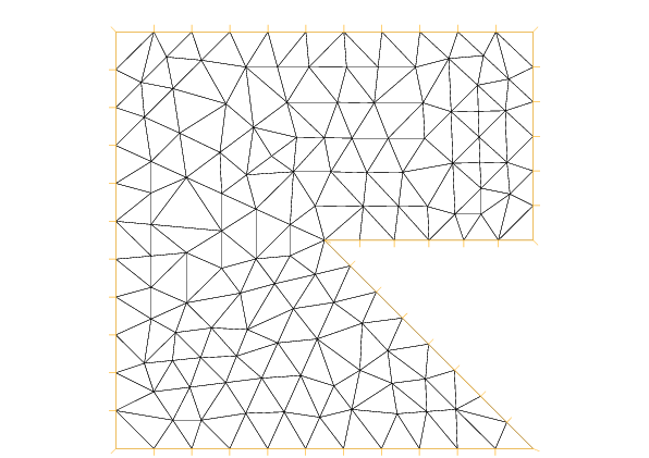
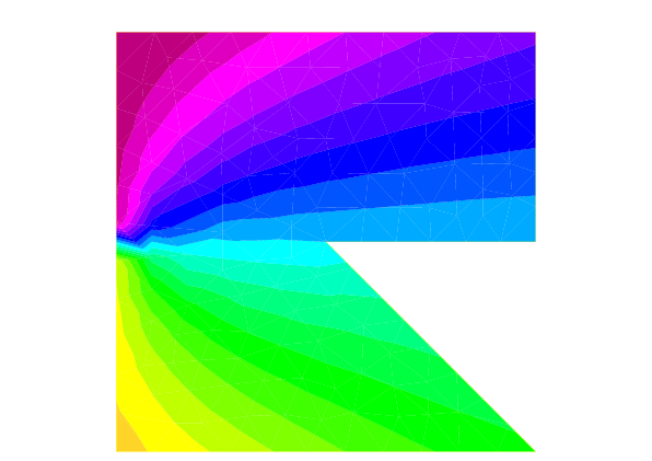
TEST02B defines the "reentrant corner" problem, using an angle of OMEGA = 5 PI /4.

• test02b.edp, the input file.
• test02b.sh, runs FreeFem++ on the input file.
• test02b_output.txt, the output file.
• test02b_mesh.png, a PNG image of the mesh.
• test02b_u.png, a PNG image of a contour plot of the solution.

TEST02C defines the "reentrant corner" problem, using an angle of OMEGA = 6 PI /4.

• test02c.edp, the input file.
• test02c.sh, runs FreeFem++ on the input file.
• test02c_output.txt, the output file.
• test02c_mesh.png, a PNG image of the mesh.
• test02c_u.png, a PNG image of a contour plot of the solution.

TEST02D defines the "reentrant corner" problem, using an angle of OMEGA = 7 PI /4.

• test02d.edp, the input file.
• test02d.sh, runs FreeFem++ on the input file.
• test02d_output.txt, the output file.
• test02d_mesh.png, a PNG image of the mesh.
• test02d_u.png, a PNG image of a contour plot of the solution.

TEST02E defines the "reentrant corner" problem, using an angle of OMEGA = 8 PI /4.

• test02e.edp, the input file.
• test02e.sh, runs FreeFem++ on the input file.
• test02e_output.txt, the output file.
• test02e_mesh.png, a PNG image of the mesh.
• test02e_u.png, a PNG image of a contour plot of the solution.

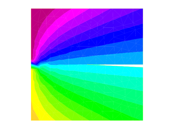
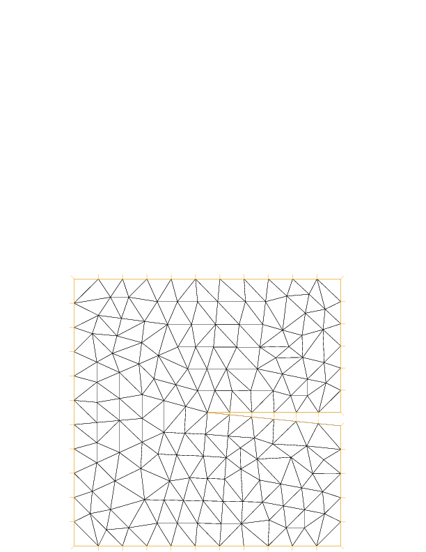
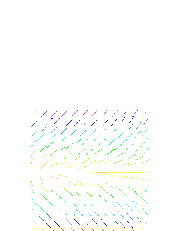
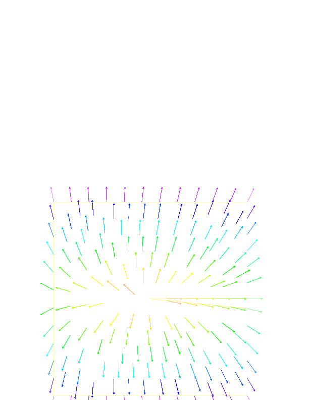
TEST03a defines the "linear elasticity" problem, a coupled system of two equations with a mixed derivative in the coupling term, defined on the [-1,+1]x[-1,+1] square, with a slit from (0,0) to (1,0), using parameter values nu = 0.3, E = 1, lambda = 0.5444837367825, Q = 0.5430755788367.

• test03a.edp, the input file.
• test03a.sh, runs FreeFem++ on the input file.
• test03a_output.txt, the output file.
• test03a_mesh.png, a PNG image of the mesh.
• test03a_u.png, a PNG image of a vector plot of the solution.

TEST03b defines the "linear elasticity" problem, a coupled system of two equations with a mixed derivative in the coupling term, defined on the [-1,+1]x[-1,+1] square, with a slit from (0,0) to (1,0), using parameter values nu = 0.3, E = 1, lambda = 0.9085291898461, Q = -0.2189232362488.

• test03b.edp, the input file.
• test03b.sh, runs FreeFem++ on the input file.
• test03b_output.txt, the output file.
• test03b_mesh.png, a PNG image of the mesh.
• test03b_u.png, a PNG image of a vector plot of the solution.

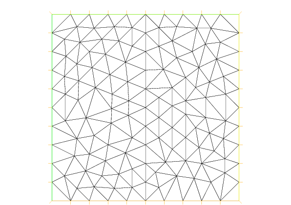
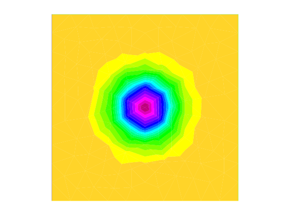
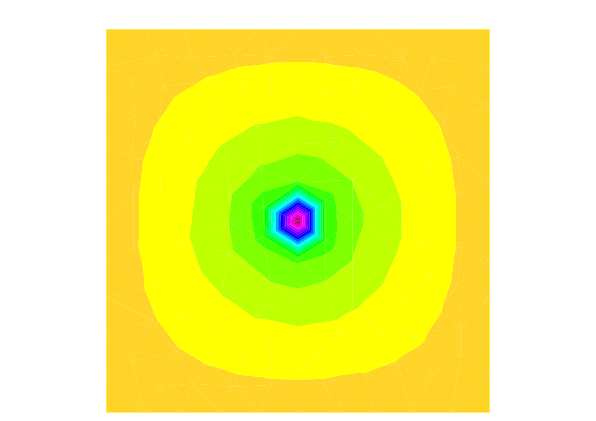
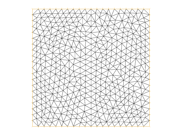
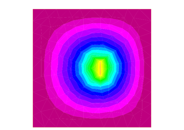
TEST04a defines the "peak" problem on the [0,+1]x[0,+1] square, using parameters XC = 0.5, YC = 0.5, ALPHA = 1000.

• test04a.edp, the input file.
• test04a.sh, runs FreeFem++ on the input file.
• test04a_output.txt, the output file.
• test04a_mesh.png, a PNG image of the mesh.
• test04a_u.png, a PNG image of a contour plot of the solution.

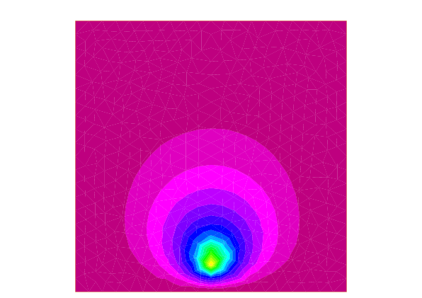
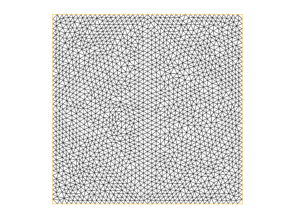
TEST04b defines the "peak" problem on the [0,+1]x[0,+1] square, using parameters XC = 0.51, YC = 0.117, ALPHA = 100000.

• test04b.edp, the input file.
• test04b.sh, runs FreeFem++ on the input file.
• test04b_output.txt, the output file.
• test04b_mesh.png, a PNG image of the mesh.
• test04b_u.png, a PNG image of a contour plot of the solution.

TEST05 defines the "battery" problem. This problem is defined on a rectangle which has been subdivided into seven subregions. Because of the complicated internal walls, it was expedient to create the mesh beforehand with BAMG.

• battery_g.msh, the BAMG geometry file file.
• battery_o.msh, the BAMG mesh file.
• battery_convert.edp, a FreeFem++ script which converts the BAMG geometry and mesh files into a FreeFem++ mesh file.
• battery.msh, the FreeFem++ mesh file.
• test05.edp, the input file.
• test05.sh, runs FreeFem++ on the input file.

TEST06A defines the "boundary layer" problem on the [-1,+1]x[-1,+1] square, using the parameter EPS = 0.1.

• test06a.edp, the input file.
• test06a.sh, runs FreeFem++ on the input file.
• test06a_output.txt, the output file.
• test06a_mesh.png, a PNG image of the mesh.
• test06a_u.png, a PNG image of a contour plot of the solution.

TEST06B defines the "boundary layer" problem on the [-1,+1]x[-1,+1] square, using the parameter EPS = 0.001. The only difference from TEST06A is the value of EPS, but this test fails to run at all. Even EPS=0.01 won't run.

• test06b.edp, the input file.
• test06b.sh, runs FreeFem++ on the input file.
• test06b_output.txt, the output file.
• test06b_mesh.png, a PNG image of the mesh.
• test06b_u.png, a PNG image of a contour plot of the solution.

TEST07 defines the "boundary line singularity" problem on the [0,+1]x[0,+1] square. There is a singularity in the right hand side function F(X,Y), at the left boundary. We use the parameter value ALPHA = 0.6.

• test07.edp, the input file.
• test07.sh, runs FreeFem++ on the input file.
• test07_output.txt, the output file.
• test07_mesh.png, a PNG image of the mesh.
• test07_u.png, a PNG image of a contour plot of the solution.

TEST08a defines the "oscillatory" problem on the [0,+1]x[0,+1] square, using parameter ALPHA = 1 / ( 10 * PI ).

• test08a.edp, the input file.
• test08a.sh, runs FreeFem++ on the input file.
• test08a_output.txt, the output file.
• test08a_mesh.png, a PNG image of the mesh.
• test08a_u.png, a PNG image of a contour plot of the solution.

TEST08b defines the "oscillatory" problem on the [0,+1]x[0,+1] square, using parameter ALPHA = 1 / ( 50 * PI ).

• test08b.edp, the input file.
• test08b.sh, runs FreeFem++ on the input file.
• test08b_output.txt, the output file.
• test08b_mesh.png, a PNG image of the mesh.
• test08b_u.png, a PNG image of a contour plot of the solution.

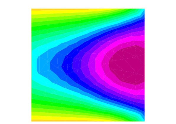
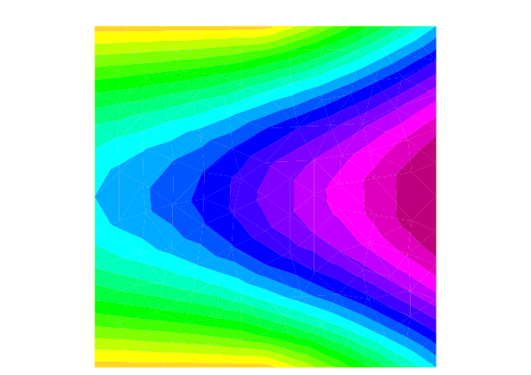
TEST09a defines the "wave front" problem on the [0,+1]x[0,+1] square with parameters ALPHA = 20, XC = -0.05, YC = -0.05, R0 = 0.7.

• test09a.edp, the input file.
• test09a.sh, runs FreeFem++ on the input file.
• test09a_output.txt, the output file.
• test09a_mesh.png, a PNG image of the mesh.
• test09a_u.png, a PNG image of a contour plot of the solution.

TEST09b defines the "wave front" problem on the [0,+1]x[0,+1] square with parameters ALPHA = 1000, XC = -0.05, YC = -0.05, R0 = 0.7.

• test09b.edp, the input file.
• test09b.sh, runs FreeFem++ on the input file.
• test09b_output.txt, the output file.
• test09b_mesh.png, a PNG image of the mesh.
• test09b_u.png, a PNG image of a contour plot of the solution.

TEST09c defines the "wave front" problem on the [0,+1]x[0,+1] square with parameters ALPHA = 1000, XC = 1.5, YC = 0.25, R0 = 0.92.

• test09c.edp, the input file.
• test09c.sh, runs FreeFem++ on the input file.
• test09c_output.txt, the output file.
• test09c_mesh.png, a PNG image of the mesh.
• test09c_u.png, a PNG image of a contour plot of the solution.

TEST09d defines the "wave front" problem on the [0,+1]x[0,+1] square with parameters ALPHA = 50, XC = 0.5, YC = 0.5, R0 = 0.25.

• test09d.edp, the input file.
• test09d.sh, runs FreeFem++ on the input file.
• test09d_output.txt, the output file.
• test09d_mesh.png, a PNG image of the mesh.
• test09d_u.png, a PNG image of a contour plot of the solution.

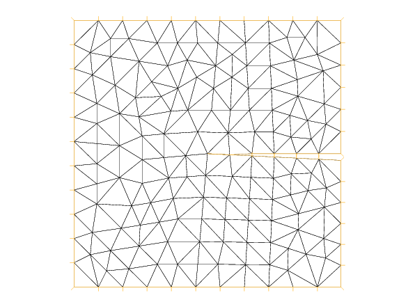
TEST10a defines the "interior line singularity" problem on the [-1,+1]x[-1,+1] square with parameters ALPHA = 2.5, BETA = 0.0.

• test10a.edp, the input file.
• test10a.sh, runs FreeFem++ on the input file.
• test10a_output.txt, the output file.
• test10a_mesh.png, a PNG image of the mesh.
• test10a_u.png, a PNG image of a contour plot of the solution.

TEST10b defines the "interior line singularity" problem on the [-1,+1]x[-1,+1] square with parameters ALPHA = 1.1, BETA = 0.0.

• test10b.edp, the input file.
• test10b.sh, runs FreeFem++ on the input file.
• test10b_output.txt, the output file.
• test10b_mesh.png, a PNG image of the mesh.
• test10b_u.png, a PNG image of a contour plot of the solution.

TEST10c defines the "interior line singularity" problem on the [-1,+1]x[-1,+1] square with parameters ALPHA = 1.5, BETA = 0.6.

• test10c.edp, the input file.
• test10c.sh, runs FreeFem++ on the input file.
• test10c_output.txt, the output file.
• test10c_mesh.png, a PNG image of the mesh.
• test10c_u.png, a PNG image of a contour plot of the solution.

TEST11 defines the "intersecting interfaces" problem on the [-1,+1]x[-1,+1] square.

• test11.edp, the input file.
• test11.sh, runs FreeFem++ on the input file.
• test11_output.txt, the output file.
• test11_mesh.png, a PNG image of the mesh.
• test11_u.png, a PNG image of a contour plot of the solution.

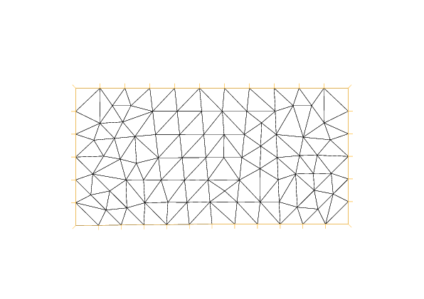
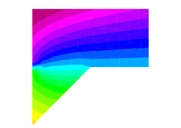
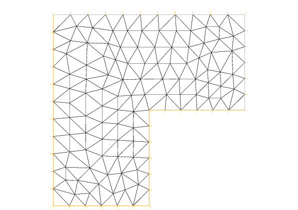
TEST12 defines the "multiple difficulties" problem, on the "upside down L" shaped region.

• test12.edp, the input file.
• test12.sh, runs FreeFem++ on the input file.

You can go up one level to the Examples directory.