

Section 1.2 Geometric View
Subsection 1.2.1 Geometric representation of a vector
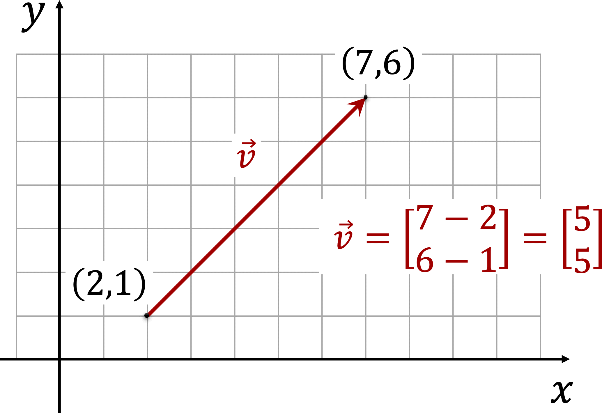
As describe in Section 1.1, we define a vector in a column form.
- The coordinate in the first row corresponds to the difference between the \(x-\)coordinates of the tail and head of the vector.
- The coordinate in the second row corresponds to the difference between the \(y-\)coordinates of the tail and head of the vector.
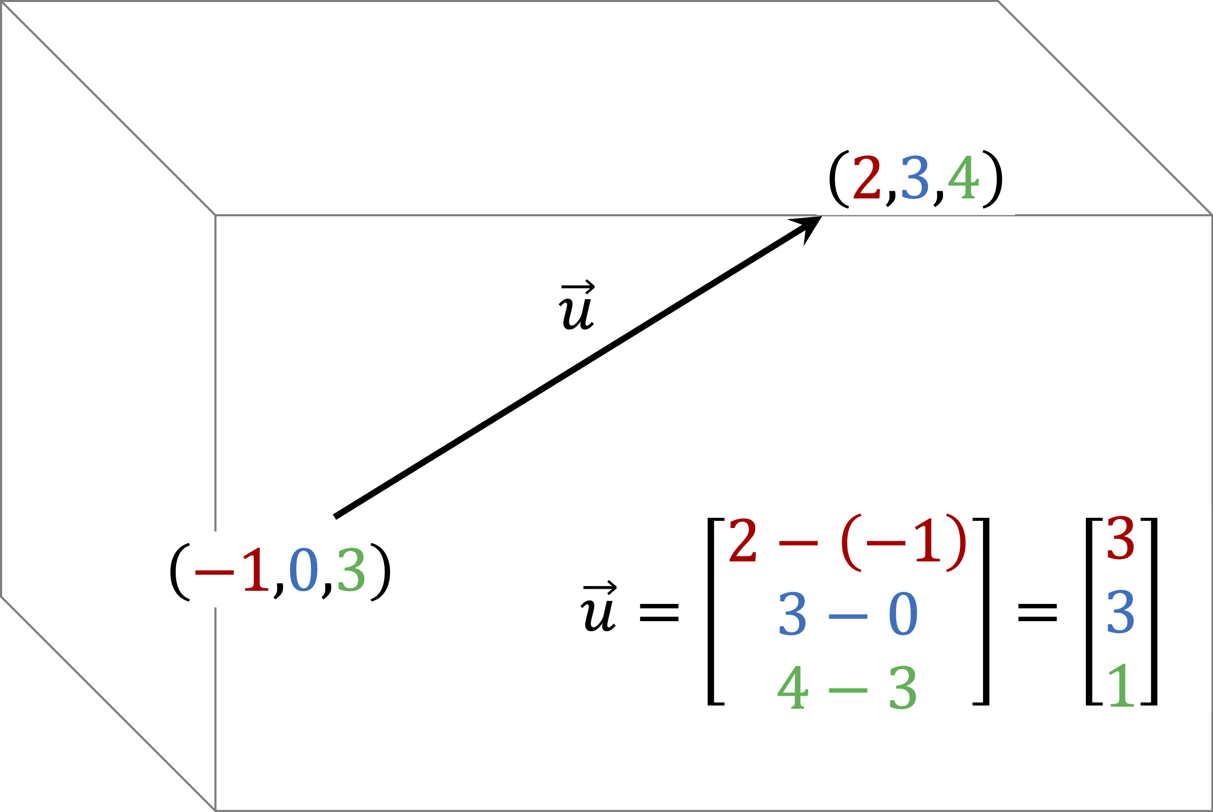
- The coordinate in the third row corresponds to the difference between the \(z-\)coordinates of the tail and head of the vector.
Example 1.2.2. Vector coordinates in 3D.
Insight 1.2.3. Equivalent Vectors.
A Vector is completely defined by two quantities: magnitude and orientation. Any two vectors that have the same magnitude and orientation are said to be equal.
As long as the differences between coordinates are the same, we consider vectors to be equal. In the example below, all the vectors shown are equivalent, independently of where they are located in the plane.
Example 1.2.4. Equivalent vectors.
\begin{equation*}
\begin{array}{lcllcllclcl}
A \amp = \amp (0,0), \amp B \amp = \amp (3,2), \amp \vec{v}_1 \amp =\amp \left[\begin{array}{r} 3-0 \\ 2-0 \end{array}\right]\amp =\amp \left[\begin{array}{r} 3 \\ 2 \end{array}\right]\\
\amp \amp \amp \amp \amp \amp \amp \amp \amp \amp\\
A \amp = \amp (4,1), \amp B \amp = \amp (7,3), \amp \vec{v}_2 \amp =\amp \left[\begin{array}{r} 7-4 \\ 3-1 \end{array}\right]\amp =\amp \left[\begin{array}{r} 3 \\ 2 \end{array}\right]\\
\amp \amp \amp \amp \amp \amp \amp \amp \amp \amp\\
A \amp = \amp (-5,2), \amp B \amp = \amp (-2,4), \amp \vec{v}_3 \amp =\amp \left[\begin{array}{r} -2+5 \\ 4-2 \end{array}\right]\amp =\amp \left[\begin{array}{r} 3 \\ 2 \end{array}\right]\\
\amp \amp \amp \amp \amp \amp \amp \amp \amp \amp\\
A \amp = \amp (-7,-4), \amp B \amp = \amp (-4,-2), \amp \vec{v}_4 \amp =\amp \left[\begin{array}{r} -4+7 \\ -2+4 \end{array}\right]\amp =\amp \left[\begin{array}{r} 3 \\ 2 \end{array}\right]\\
\amp \amp \amp \amp \amp \amp \amp \amp \amp \amp\\
A \amp = \amp (3,-2), \amp B \amp = \amp (6,0), \amp \vec{v}_5 \amp =\amp \left[\begin{array}{r} 6-3 \\ 0+2 \end{array}\right]\amp =\amp \left[\begin{array}{r} 3 \\ 2 \end{array}\right]\\
\amp \amp \amp \amp \amp \amp \amp \amp \amp \amp\\
A \amp = \amp (2.5,1.5), \amp B \amp = \amp (5.5,3.5), \amp \vec{v}_6 \amp =\amp \left[\begin{array}{r} 5.5-2.5 \\ 3.5-1.5 \end{array}\right]\amp =\amp \left[\begin{array}{r} 3 \\ 2 \end{array}\right]\\
\end{array}
\end{equation*}
-
Equivalent Vectors in \(\R^2\).
-
Equivalent Vectors in \(\R^3\).
Subsection 1.2.2 Vector Addition
To add two vectors geometrically, set the tail of the second vector to the head of the first vector. The resulting vector will go from the tail of the first vector to the head of the second vector.
-
Vector Addition in \(\R^2\).
-
Vector Addition in \(\R^3\).
Subsection 1.2.3 Vector Subtraction
To subtract two vectors geometrically, flip the second vector and proceed as in the vector addition.
-
Vector Subtraction in \(\R^2\).
-
Vector Subtraction in \(\R^3\).
Subsection 1.2.4 Magnitude of a Vector
The length or magnitude of a vector is the distance between its initial and end points. Calculations of vector magnitude are discussed in section Section 1.3.
Insight 1.2.5. Unit Vectors.
A unit vector is a vector which magnitude is equal to 1. We can find a unit vector in the direction of a given vector by dividing it by its magnitude.
-
Unit Vector in \(\R^2\).\(~\)
-
Unit Vector in \(\R^3\).In the video below,the following three vectors are normalized\begin{equation*} \begin{array}{lccclcc} \vec{u}_1 \amp=\amp \left[ \begin{array}{c} 3 \\0\\0 \end{array}\right], \amp \hspace{0.5cm} \Vert \vec{u}_1\Vert = 3, \hspace{0.5cm} \amp \hat{u}_1 \amp =\amp \left[ \begin{array}{c} 1\\0\\0 \end{array}\right], \\ \vec{u}_2 \amp=\amp \left[ \begin{array}{c} 0\\-3\\3 \end{array}\right], \amp \hspace{0.5cm} \Vert \vec{u}_1\Vert = 3\sqrt{2}, \hspace{0.5cm} \amp \hat{u}_2 \amp = \amp \left[ \begin{array}{c} 0\\ -\sqrt{2}/2\\\sqrt{2}/2 \end{array}\right], \\ \vec{u}_3 \amp=\amp \left[ \begin{array}{c}-2\\3\\1 \end{array}\right], \amp \hspace{0.5cm}\Vert \vec{u}_1\Vert = \sqrt{14}, \hspace{0.5cm} \amp \hat{u}_3 \amp =\amp \left[ \begin{array}{c} -\sqrt{14}/7\\ 3 \sqrt{14}/14\\ \sqrt{14}/14 \end{array}\right]. \end{array} \end{equation*}
Subsection 1.2.5 Orientation of a Vector
The orientation of a 2D vector is given by the angle it makes with the positive \(x-\) axis. Calculations of vector orientation are discussed in section Section 1.3.
