LCVT_DATASET
Latin Hypercubes using CVT Startup

LCVT_DATASET is a FORTRAN90 program which computes a Latin Hypercube in M dimensions, with N points, using a CVT dataset as the initial estimate, and can write it to a file.

A Latin Square dataset is typically a two dimensional dataset of N points in the unit square, with the property that, if both the x and y axes are divided up into N equal subintervals, exactly one dataset point has an x or y coordinate in each subinterval. Latin squares can easily be extended to the case of M dimensions, and may be pedantically called Latin Hypersquares or Latin Hypercubes in such a case. Statisticians like Latin Squares, as do experiment designers, and and people who need to approximate scalar functions of many variables.

The fact that the projection of a Latin Square dataset onto any coordinate axis is either exactly evenly spaced, or approximately so (depending on the algorithm), turns out to be an attractive feature for many uses.

However, a CVT dataset in a regular domain, such as the unit hypercube, has the tendency for the projections of the points to cluster together in any coordinate axis. This program is mainly an attempt to explore whether a dataset can be computed using techniques similar to those of a CVT, but with the constraint (whether imposed or expected) that the point projections do not clump up.

The approach used here is quite simple. First we compute a CVT in M dimensions, comprising N points. We assume that the bounding region is the unit hypercube. We are now going to adjust the coordinates of the points to achieve the Latin Hypercube property. For each coordinate direction, we simply sort the points by that coordinate, and then overwrite the original values by the values we'd expect to get for a centered Latin Hypercube, namely, 1/(2*N), 3/(2*N), ..., (2*N-1)/(2*N).

Now this process guarantees that we get a Latin Hypercube. Our hope is that the process of adjusting the point coordinates does not too severely damage the nice dispersion properties inherent in the CVT point placement.

An earlier version of this program was "very" interactive, allowing the user to enter input in any order. This turned out to be a little too confusing. The new version of the program asks the user for input in a strict order. If you find this procedure too restrictive, you can try out the old program.

Briefly the user needs to specify the following:

1. The spatial dimension M of the points;
2. The number of points N to be generated.
3. The random number seed;
4. How the initial points are chosen. If you have no preference, choose UNIFORM.
   • GRID, use a grid of points;
   • HALTON, use Halton points;
   • RANDOM, use RANDOM_NUMBER (Fortran90 intrinsic);
   • UNIFORM, use a simple uniform random number generator;
   • USER, call the "user" routine;
   • (file_name), read the initial points from a file.
5. The number of CVT iterations. If you have no preference, try 5, 10 or 20;
6. How the sampling is done. If you have no preference, use UNIFORM.
   • GRID, use a grid of points;
   • HALTON, use Halton points;
   • RANDOM, use RANDOM_NUMBER (Fortran90 intrinsic);
   • UNIFORM, use a simple uniform random number generator;
   • USER, call the "user" routine;
7. The number of sampling points to use. Think of this as a sampling of the unit hypercube. So to compare it to N, the number of points, you need to take its M-th root. In 2D, if you're using 10 generators, and 100 sample points, to get area and sampling computations twice as good requires 4 times the sampling. It never hurts to use more sampling points.
8. The "batch size". This parameter controls how many sampling points are to be generated at one time. You can set this value equal to the number of sampling points, but if you are having memory problems, it can be set lower. In such a case, a smaller value might be 1000, for instance.
9. The number of CVT iterations to carry out. It's not really necessary to compute the CVT super accurately, since we're just going to perturb it anyway. This value could be anywhere from 10 to 500. Convergence of the CVT is typically slow, especially if the starting positions are poor.
10. The number of Latin Hypercube iterations to carry out. Actually, the iterations don't seem to improve the data much, so a value of 1 or 2 can be reasonable.
11. The name of a file into which the final pointset should be written.

Licensing:

The computer code and data files described and made available on this web page are distributed under the GNU LGPL license.

Languages:

LCVT_DATASET is available in a C++ version and a FORTRAN90 version and a MATLAB version.

Related Data and Programs:

CVT, a FORTRAN90 library which computes a CVT (Centroidal Voronoi Tessellation).

CVT_DATASET, a FORTRAN90 program which can compute a CVT (Centroidal Voronoi Tessellation).

FAURE_DATASET, a FORTRAN90 program which creates a Faure quasirandom dataset;

GRID_DATASET, a FORTRAN90 program which creates a grid sequence and writes it to a file.

LATIN_CENTER_DATASET, a FORTRAN90 program which creates a Latin Center Hypercube dataset;

LATIN_EDGE_DATASET, a FORTRAN90 program which creates a Latin Edge Hypercube dataset;

LATIN_RANDOM_DATASET, a FORTRAN90 program which creates a Latin Random Hypercube dataset;

LCVT, a FORTRAN90 library which is used by LCVT_DATASET; a compiled copy of that library must be available to build the program.

LCVT, a dataset directory which contains a collection of sample LCVT datasets created by LCVT_DATASET.

NIEDERREITER2_DATASET, a FORTRAN90 program which creates a Niederreiter quasirandom dataset with base 2;

NORMAL_DATASET, a FORTRAN90 program which generates a dataset of multivariate normal pseudorandom values and writes them to a file.

SOBOL_DATASET, a FORTRAN90 program which computes a Sobol quasirandom sequence and writes it to a file.

TABLE_LATINIZE, a FORTRAN90 program which can read a TABLE file of points and "latinize" the points, that is, "gently" rearranging them so that they are regularly spaced in every coordinate direction.

TABLE_QUALITY, a FORTRAN90 program which can read a TABLE file of points and compute various measures of the quality of dispersion.

TABLE_TOP, a FORTRAN90 program which can read a TABLE file of points in M dimensions (where M is likely to be more than 2!) and make plots of all 2D projections onto pairs of coordinate axes.

UNIFORM_DATASET, a FORTRAN90 program which generates a dataset of multivariate uniform pseudorandom values and writes them to a file.

VAN_DER_CORPUT_DATASET, a FORTRAN90 program which creates a van der Corput quasirandom sequence and writes it to a file.

Reference:

1. Franz Aurenhammer,
   Voronoi diagrams - a study of a fundamental geometric data structure,
   ACM Computing Surveys,
   Volume 23, Number 3, September 1991, pages 345-405.
2. Franz Aurenhammer, Rolf Klein,
   Voronoi Diagrams,
   in Handbook of Computational Geometry,
   edited by J Sack, J Urrutia,
   Elsevier, 1999,
   LC: QA448.D38H36.
3. John Burkardt, Max Gunzburger, Janet Peterson, Rebecca Brannon,
   User Manual and Supporting Information for Library of Codes for Centroidal Voronoi Placement and Associated Zeroth, First, and Second Moment Determination,
   Sandia National Laboratories Technical Report SAND2002-0099,
   February 2002,
   ../../publications/bgpb_2002.pdf
4. Qiang Du, Vance Faber, Max Gunzburger,
   Centroidal Voronoi Tessellations: Applications and Algorithms,
   SIAM Review,
   Volume 41, Number 4, December 1999, pages 637-676.
5. Michael McKay, William Conover, Richard Beckman,
   A Comparison of Three Methods for Selecting Values of Input Variables in the Analysis of Output From a Computer Code,
   Technometrics,
   Volume 21, 1979, pages 239-245.
6. Vicente Romero, John Burkardt, Max Gunzburger, Janet Peterson,
   Initial Evaluation of Pure and "Latinized" Centroidal Voronoi Tessellation for Non-Uniform Statistical Sampling,
   Sensitivity Analysis of Model Output (SAMO 2004) Conference, Santa Fe, March 8-11, 2004,
   rbgp_2004.pdf.
7. Yuki Saka, Max Gunzburger, John Burkardt,
   Latinized, improved LHS, and CVT point sets in hypercubes,
   submitted to IEEE Transactions on Information Theory,
   sgb_submitted.pdf.

Source Code:

• lcvt_dataset.f90, the source code.
• lcvt_dataset_old.f90, the older version of the source code.

Examples and Tests:

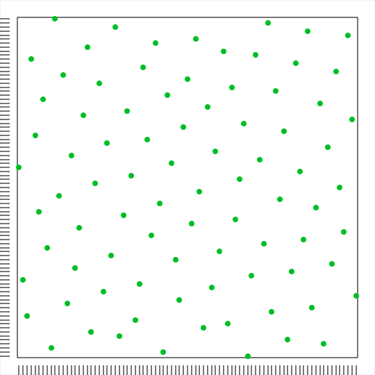
Example 1 is a dataset of N=85 points with spatial dimension M=2, using UNIFORM initialization and sampling, and 10,000 sample points:

• lcvt01_input.txt, input commands.
• lcvt01.txt, printed output.
• lcvt01.txt, the LCVT dataset.
• lcvt01.png, a PNG image of the LCVT dataset, created by PLOT_POINTS.

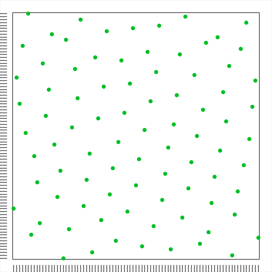
Example 2 is a dataset of N=85 points with spatial dimension M=2, using RANDOM initialization and sampling, and 1000000 sample points:

• lcvt02_input.txt, input commands.
• lcvt02.txt, printed output.
• lcvt02.txt, the LCVT dataset.
• lcvt02.png, a PNG image of the LCVT dataset, created by PLOT_POINTS.

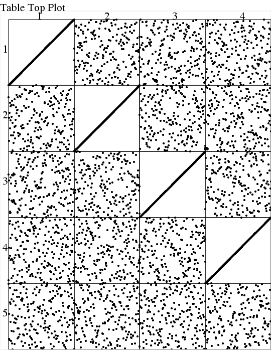
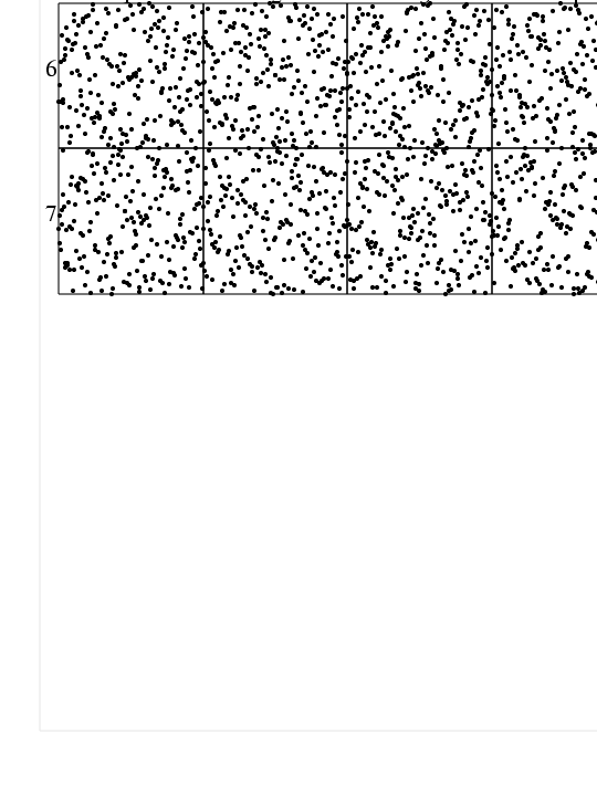
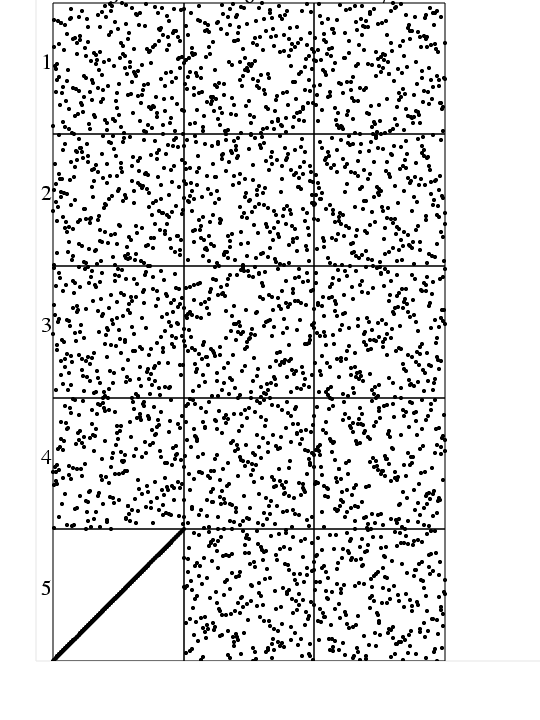
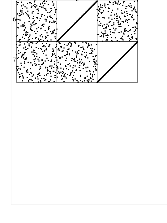
Example 3 is a dataset of N=200 points with spatial dimension M=7, using UNIFORM initialization and sampling, and 20,000 sample points, 5 CVT iterations and 2 Latinization iterations:

• lcvt03_input.txt, input commands.
• lcvt03.txt, printed output.
• lcvt03.txt, the LCVT dataset.
• lcvt03_page1.png, "page 1" of a PNG image of pairs of coordinates of the LCVT dataset, created by TABLE_TOP.
• lcvt03_page2.png, "page 2" of a PNG image of pairs of coordinates of the LCVT dataset, created by TABLE_TOP.
• lcvt03_page3.png, "page 3" of a PNG image of pairs of coordinates of the LCVT dataset, created by TABLE_TOP.
• lcvt03_page4.png, "page 4" of a PNG image of pairs of coordinates of the LCVT dataset, created by TABLE_TOP.

List of Routines:

• LCVT_DATASET generates a CVT dataset and writes it to a file.
• CH_CAP capitalizes a single character.
• CH_EQI is a case insensitive comparison of two characters for equality.
• CH_TO_DIGIT returns the integer value of a base 10 digit.
• CLUSTER_ENERGY returns the energy of a dataset.
• CVT_ITERATION takes one step of the CVT iteration.
• FILE_COLUMN_COUNT counts the number of columns in the first line of a file.
• FILE_ROW_COUNT counts the number of row records in a file.
• FIND_CLOSEST finds the Voronoi cell generator closest to a point X.
• GET_SEED returns a seed for the random number generator.
• GET_UNIT returns a free FORTRAN unit number.
• I4_TO_HALTON computes an element of a vector Halton sequence.
• LCVT_WRITE writes a Latinized CVT dataset to a file.
• PARAM_PRINT prints the program parameters.
• PRIME returns any of the first PRIME_MAX prime numbers.
• R8_UNIFORM_01 returns a unit pseudorandom R8.
• R8MAT_LATINIZE "Latinizes" an R8MAT.
• R8TABLE_DATA_READ reads data from an R8TABLE file.
• R8VEC_SORT_HEAP_INDEX_A does an indexed heap ascending sort of an R8VEC.
• REGION_SAMPLER returns a sample point in the physical region.
• S_BLANK_DELETE removes blanks from a string, left justifying the remainder.
• S_CAP replaces any lowercase letters by uppercase ones in a string.
• S_EQI is a case insensitive comparison of two strings for equality.
• S_TO_R8 reads an R8 value from a string.
• S_TO_R8VEC reads an R8VEC from a string.
• S_WORD_COUNT counts the number of "words" in a string.
• TEST_REGION determines if a point is within the physical region.
• TIMESTAMP prints the current YMDHMS date as a time stamp.
• TIMESTRING writes the current YMDHMS date into a string.
• TUPLE_NEXT_FAST computes the next element of a tuple space, "fast".

You can go up one level to the FORTRAN90 source codes.