FD1D_WAVE is a FORTRAN77 program which applies the finite difference method to solve a version of the wave equation in one spatial dimension.
The wave equation considered here is an extremely simplified model of the physics of waves. Many facts about waves are not modeled by this simple system, including that wave motion in water can depend on the depth of the medium, that waves tend to disperse, and that waves of different frequency may travel at different speeds. However, as a first model of wave motion, the equation is useful because it captures a most interesting feature of waves, that is, their usefulness in transmitting signals.
This program solves the 1D wave equation of the form:
Utt = c^2 Uxx
over the spatial interval [X1,X2] and time interval [T1,T2],
with initial conditions:
        U(T1,X)  = U_T1(X),
        Ut(T1,X) = UT_T1(X),
and boundary conditions of Dirichlet type:
        U(T,X1) = U_X1(T),

        U(T,X2) = U_X2(T).
The value C represents the propagation speed of waves.
The program uses the finite difference method, and marches forward in time, solving for all the values of U at the next time step by using the values known at the previous two time steps.
Central differences may be used to approximate both the time and space derivatives in the original differential equation.
Thus, assuming we have available the approximated values of U at the current and previous times, we may write a discretized version of the wave equation as follows:
        Uxx(T,X) = ( U(T,   X+dX) - 2 U(T,X) + U(T,   X-dX) ) / dX^2
        Utt(T,X) = ( U(T+dt,X   ) - 2 U(T,X) + U(T-dt,X   ) ) / dT^2
If we multiply the first term by C^2 and solve for the single
unknown value U(T+dt,X), we have:
        U(T+dT,X) =        (     C^2 * dT^2 / dX^2 ) * U(T,   X+dX)
                    +  2 * ( 1 - C^2 * dT^2 / dX^2 ) * U(T,   X   )
                    +      (     C^2 * dT^2 / dX^2 ) * U(T,   X-dX)
                    -                                  U(T-dT,X   )
(Equation to advance from time T to time T+dT, except for FIRST step!)
However, on the very first step, we only have the values of U for the initial time, but not for the previous time step. In that case, we use the initial condition information for dUdT which can be approximated by a central difference that involves U(T+dT,X) and U(T-dT,X):
dU/dT(T,X) = ( U(T+dT,X) - U(T-dT,X) ) / ( 2 * dT )
and so we can estimate U(T-dT,X) as
U(T-dT,X) = U(T+dT,X) - 2 * dT * dU/dT(T,X)
If we replace the "missing" value of U(T-dT,X) by the known values
on the right hand side, we now have U(T+dT,X) on both sides of the
equation, so we have to rearrange to get the formula we use
for just the first time step:
        U(T+dT,X) =   1/2 * (     C^2 * dT^2 / dX^2 ) * U(T,   X+dX)
                    +       ( 1 - C^2 * dT^2 / dX^2 ) * U(T,   X   )
                    + 1/2 * (     C^2 * dT^2 / dX^2 ) * U(T,   X-dX)
                    +  dT *                         dU/dT(T,   X   )
(Equation to advance from time T to time T+dT for FIRST step.)
It should be clear now that the quantity ALPHA = C * DT / DX will affect the stability of the calculation. If it is greater than 1, then the middle coefficient 1-C^2 DT^2 / DX^2 is negative, and the sum of the magnitudes of the three coefficients becomes unbounded.
The computer code and data files described and made available on this web page are distributed under the GNU LGPL license.
FD1D_WAVE is available in a C version and a C++ version and a FORTRAN77 version and a FORTRAN90 version and a MATLAB version.
FD1D_ADVECTION_LAX, a FORTRAN77 program which applies the finite difference method to solve the time-dependent advection equation ut = - c * ux in one spatial dimension, with a constant velocity, using the Lax method to treat the time derivative.
FD1D_BURGERS_LAX, a FORTRAN77 program which applies the finite difference method and the Lax-Wendroff method to solve the non-viscous time-dependent Burgers equation in one spatial dimension.
FD1D_BURGERS_LEAP, a FORTRAN77 program which applies the finite difference method and the leapfrog approach to solve the non-viscous time-dependent Burgers equation in one spatial dimension.
FD1D_BVP, a FORTRAN77 program which applies the finite difference method to a two point boundary value problem in one spatial dimension.
FD1D_HEAT_EXPLICIT, a FORTRAN77 program which uses the finite difference method and explicit time stepping to solve the time dependent heat equation in 1D.
FD1D_HEAT_IMPLICIT, a FORTRAN77 program which uses the finite difference method and implicit time stepping to solve the time dependent heat equation in 1D.
FD1D_HEAT_STEADY, a FORTRAN77 program which uses the finite difference method to solve the steady (time independent) heat equation in 1D.
FD1D_PREDATOR_PREY, a FORTRAN77 program which implements a finite difference algorithm for predator-prey system with spatial variation in 1D.
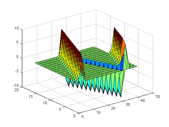
test01_plot sets up the "shark wave".
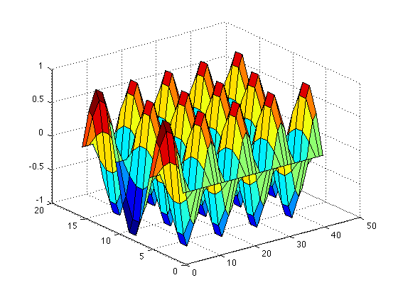
test02_plot sets up a sine wave.
You can go up one level to the FORTRAN77 source codes.