

Section 1.2 Elementary Operations and Reduced Forms
Objectives
-
Understand row operations in matrices.
-
Determine if two matrices are row equivalent.
-
Understand row-echelon and reduced row-echelon forms.
-
Use row operations to convert a matrix to its reduced row-echelon form.
\(\, \)
\(\Large{\textbf{Section Content}} \)
\(\, \)
Subsection 1.1.1 Elementary row operations
Elementary row operations are element-wise operations applied to a given row in a matrix.
There are three main types of elementary row operations:
-
Interchange two rows of a matrix.
This is the equivalent to interchanging two equations in a system of equations. The notation for this operation is \(R_i \leftrightarrow R_j \) where \(i \) and \(j \) are the two rows to be interchanged.\begin{equation*} \, \end{equation*}\begin{equation*} \, \end{equation*} -
Multiply the elements of a row by a nonzero constant.
This is the equivalent of multiplying both sides of an equation by a non-zero constant. The notation for this operation is \(R_i \rightarrow k R_i \) where \(i \) the row in question and \(k \) the constant.\begin{equation*} \, \end{equation*}\begin{equation*} \, \end{equation*} -
Add a multiple of the elements of one row to the corresponding elements of another row.
This is the equivalent to adding a multiple of one equation to another equation. The notation for this operation is \(R_i \rightarrow R_i + k R_j \) where \(i \) the row to be changed, \(j \) is the row used for the operations but not to be changed, and \(k \) the constant.\begin{equation*} \, \end{equation*}\begin{equation*} \, \end{equation*}
Checkpoint 1.1.1. Practice elementary row operations.
Consider the matrix,
After performing the row operation \(R_2 \rightarrow R_2 - R_1\text{,}\) the new matrix is:
| \(\,\) | \(\lceil\) | -4 | 3 | -4 | 4 | \(\rceil\) |
| \(\boldsymbol{A} =\) | \(\vert\) | \(\vert\) | ||||
| \(\,\) | \(\lfloor\) | 2 | -3 | -3 | -4 | \(\rfloor\) |
| \(\,\) | \(\,\) | \(\,\) | \(\,\) |
\(\,\)
\(8\)
\(-4\)
\(8\)
\(-7\)
To find the new \(R_2:\)
Checkpoint 1.1.2. Practice elementary row operations.
Consider the matrix,
Perform the row operation \(R_1 \rightarrow R_1 + \frac{1}{2}R_3\text{.}\) The new matrix is:
| \(\,\) | \(\lceil\) | \(\rceil\) | ||||
| \(\boldsymbol{A} =\) | \(\vert\) | \(\vert\) | ||||
| \(\,\) | \(\lfloor\) | \(\rfloor\) | ||||
| \(\,\) | \(\,\) | \(\,\) | \(\,\) |
\(\,\)
\(-7\)
\(3\)
\(-2\)
\(-4\)
\(4\)
\(4\)
\(1\)
\(-2\)
\(-8\)
\(8\)
\(-6\)
\(-10\)
To find the new \(R_1:\)
\(\, \)
Definition 1.1.3. Row equivalency.
Two matrices are equivalent if one can be transformed into the other with a sequence of elementary row operations.
Checkpoint 1.1.4. Determine if two matrices are row equivalent.
Are the two given matrices row equivalent?
\(\,\)
-
Yes
-
No
\(\,\)
-
Yes
-
No
\(\text{Yes}\)
\(\text{No}\)
-
Yes: the second matrix is obtained after performing the row operation \(R_2 \rightarrow 2 R_2\) on the first matrix.
-
No: the second matrix is obtained by eliminating the last column from the first matrix, however eliminating columns is not a elementary row operation.
Checkpoint 1.1.5. Determine if two matrices are row equivalent.
Are the two given matrices row equivalent?
\(\,\)
-
Yes
-
No
\(\,\)
-
Yes
-
No
\(\text{No}\)
\(\text{Yes}\)
-
No: at first glance it seems that the operation is \(R_4 \rightarrow -R_4\text{,}\) however the last entry of the second matrix is not the negative the last entry of the first equation. Elementary row operations have to be applied to all elements of a row.
-
Yes: the second matrix is obtained after performing the row operation \(R_1 \rightarrow R1 + 2 R_2\) on the first matrix.
Subsection 1.1.2 Reduced row-echelon form (RREF)
A matrix is in reduced echelon form if:
- Any rows consisting entirely of zeroes
are at the bottom of the matrix
- The first nonzero element of a row is 1.
This element is called a leading
1
- The leading 1 of each row is positioned
to the right of the leading 1 of the previous row
- All other elements in a column that
contains a leading 1 are zero
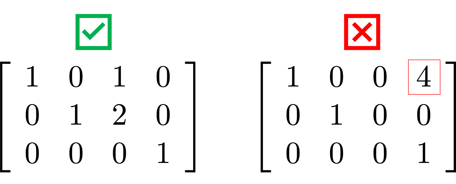
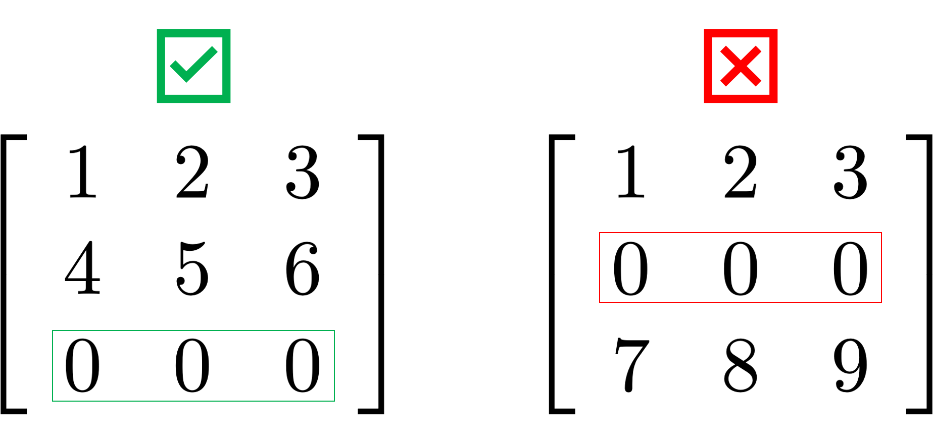
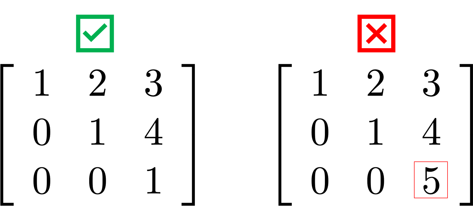
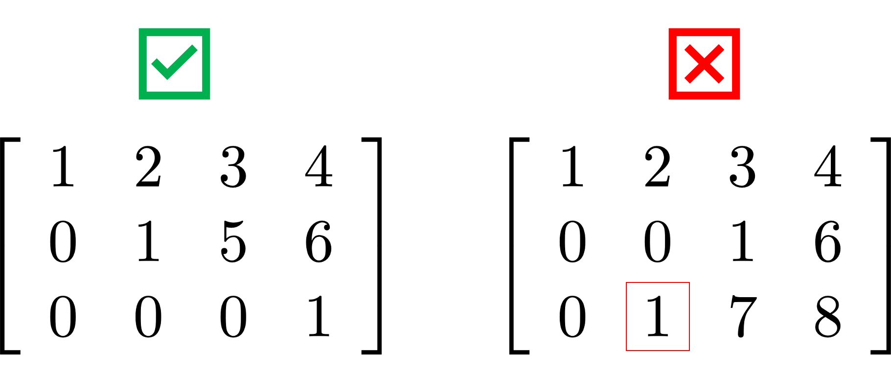
Example 1.1.6. Determine whether a matrix is RREF.
The matrix
is NOT in reduced echelon form, although it satisfies condition 1, it does not satisfies conditions 2-4.
The matrix
is NOT in reduced echelon form, although it satisfies conditions 1-3, it does not satisfies condition 4.
The matrix
is NOT in reduced echelon form, although it satisfies conditions 1-3, it does not satisfies condition 4.
The matrix
IS in reduced echelon form, it satisfies conditions 1-4.
Checkpoint 1.1.7. Difference between REF and RREF.
We can distinguish between row-echelon form (REF) and reduced row-echelon form (RREF). In short, A matrix is in REF if
- Leading nonzero entry of each row is 1.
- The leading 1 of a row is strictly to the right of the leading 1 of the row above it.
- Any all-zero rows are at the bottom of the matrix.
And in RREF if
- It is in REF
- The column of any row-leading 1 is cleared (all other entries are 0).
Determine if the following matrices are in REF, RREF or not in echelon form,
\(\,\)
-
Echelon form
-
Reduced echelon form
-
Not in echelon form
\(\,\)
-
Echelon form
-
Reduced echelon form
-
Not in echelon form
\(\,\)
-
Echelon form
-
Reduced echelon form
-
Not in echelon form
\(\text{Echelon form}\)
\(\text{Not in echelon form}\)
\(\text{Reduced echelon form}\)
-
The matrix is in echelon form (REF) but NOT in reduced echelon form (RREF) since the entries above the leading ones are not zero.
-
The matrix is not in echelon form since the first non-zero entries for rows one and two are not ones; i.e., they are not leading “ones”.
-
The matrix is in reduced echelon form (RREF). Note that not every row has to have a leading one, but those rows that do not have a leading one should be all zeros and placed at the bottom of the matrix.
Subsection 1.1.3 Convert a matrix into its reduced row-echelon form
To reduce a matrix into its RREF proceed row by row starting with row 1.
- In each row find its leading one using elementary row operations.
- After the leading one is found, use elementary row operations to set all the entries in its column equal to zero.
- Move to next row and repeat 1-2 until end of matrix
- Any row with no leading ones should consists of only zeros and it should be located at the bottom of the matrix
Example 1.1.8. Reduce a matrix into its RREF.
Consider the matrix \(A = \left[ \begin{array}{ccc} 3 \amp 6 \amp -12 \\ 2 \amp 8 \amp 0 \\ 3 \amp 1 \amp -2\\ \end{array}\right], \) find the RREF of \(A. \)
- We start by finding the leading one
in row 1, which is equivalent to making the first
entry equal to 1. To do this we divide row 1 by 3,
\begin{equation*} \left[ \begin{array}{ccc} 3 \amp 6 \amp -12 \\ 2 \amp 8 \amp 0 \\ 3 \amp 1 \amp -2\\ \end{array}\right] \hspace{1cm} R_1 \rightarrow \frac{1}{3} R_1 \hspace{1cm} \left[ \begin{array}{ccc} \color{red}{1} \amp 2 \amp -4 \\ 2 \amp 8 \amp 0 \\ 3 \amp 1 \amp -2\\ \end{array}\right] \end{equation*}
- Next, since the leading one is in
column 1, we need to set every entry in that
column equal to zero. That is, we use the newly
created leading one as a pivot. Since we are using
the one, it is easy to see that the necessary
operations are
\begin{equation*} \begin{array}{lcl} R_2 \amp \rightarrow \amp R_2 - 2R_1 \\ R_3 \amp \rightarrow \amp R_3 - 3R_1 \\ \end{array} \end{equation*}For the first operation:\begin{equation*} \begin{array}{rrrr} R_2: \amp 2 \amp 8 \amp 0 \\ -2R_1: \amp -2 \amp -4 \amp 8 \\ \hline R_2 - 2R_1 : \amp 0 \amp 4 \amp 8 \\ \end{array} \end{equation*}\begin{equation*} \left[ \begin{array}{ccc} 1 \amp 2 \amp -4 \\ 2 \amp 8 \amp 0 \\ 3 \amp 1 \amp -2\\ \end{array}\right] \hspace{1cm} R_2 \rightarrow R_2 - 2R_1 \hspace{1cm} \left[ \begin{array}{ccc} 1 \amp 2 \amp -4 \\ \color{red}{0} \amp 4 \amp 8 \\ 3 \amp 1 \amp -2\\ \end{array}\right] \end{equation*}For the second operation:\begin{equation*} \begin{array}{rrrr} R_3: \amp 3 \amp 1 \amp -2\\ -3R_1: \amp -3 \amp -6 \amp 12 \\ \hline R_3 - 3R_1 : \amp 0 \amp -5 \amp 10 \\ \end{array} \end{equation*}\begin{equation*} \left[ \begin{array}{ccc} 1 \amp 2 \amp -4 \\ 0 \amp 4 \amp 8 \\ 3 \amp 1 \amp -2\\ \end{array}\right] \hspace{1cm} R_3 \rightarrow R_3 - 3R_1 \hspace{1cm} \left[ \begin{array}{ccc} 1 \amp 2 \amp -4 \\ 0 \amp 4 \amp 8 \\ \color{red}{0} \amp -5 \amp 10 \\ \end{array}\right] \end{equation*}
- We move to next row and find its
leading one. Since the first non-zero entry is in
the second column, we make that entry equal 1. The
corresponding operation is \(R_2 \rightarrow
\frac{1}{4} R_2 \)
\begin{equation*} \left[ \begin{array}{ccc} 1 \amp 2 \amp -4 \\ 0 \amp 4 \amp 8 \\ 0 \amp -5 \amp 10 \\ \end{array}\right] \hspace{1cm} R_2 \rightarrow \frac{1}{4}R_2 \hspace{1cm} \left[ \begin{array}{ccc} 1 \amp 2 \amp -4 \\ 0 \amp \color{red}{1} \amp 2 \\ 0 \amp -5 \amp 10 \\ \end{array}\right] \end{equation*}
- The next step is to make all entries
in column 2 equal to zero. As before we use the
leading one as a pivot, so that the corresponding
operations would be,
\begin{equation*} \begin{array}{lcl} R_1 \amp \rightarrow \amp R_1 - 2R_2 \\ R_3 \amp \rightarrow \amp R_3 + 5R_2 \\ \end{array} \end{equation*}For the first operation:\begin{equation*} \begin{array}{rrrr} R_1: \amp 1 \amp 2 \amp -4 \\ -2R_2: \amp 0 \amp -2 \amp -4 \\ \hline R_1 - 2R_2 : \amp 1 \amp 0 \amp -8 \\ \end{array} \end{equation*}\begin{equation*} \left[ \begin{array}{ccc} 1 \amp 2 \amp -4 \\ 0 \amp 1 \amp 2 \\ 0 \amp -5 \amp 10 \\ \end{array}\right] \hspace{1cm} R_1 \rightarrow R_1 - 2R_2 \hspace{1cm} \left[ \begin{array}{ccc} 1 \amp \color{red}{0} \amp -8 \\ 0 \amp 1 \amp 2 \\ 0 \amp -5 \amp 10 \\ \end{array}\right] \end{equation*}For the second operation:\begin{equation*} \begin{array}{rrrr} R_3: \amp 0 \amp -5 \amp 10 \\ 5R_2: \amp 0 \amp 5 \amp 10 \\ \hline R_3 + 5R_2 : \amp 0 \amp 0 \amp 20 \\ \end{array} \end{equation*}\begin{equation*} \left[ \begin{array}{ccc} 1 \amp 0 \amp -8 \\ 0 \amp 1 \amp 2 \\ 0 \amp -5 \amp 10 \\ \end{array}\right] \hspace{1cm} R_3 \rightarrow R_3 - 3R_1 \hspace{1cm} \left[ \begin{array}{ccc} 1 \amp 0 \amp -8 \\ 0 \amp 1 \amp 2 \\ 0 \amp \color{red}{0} \amp 20 \\ \end{array}\right] \end{equation*}
- We move to next column and find its
leading one. In this case the operation is \(R_3
\rightarrow \frac{1}{20} R_3, \)
\begin{equation*} \left[ \begin{array}{ccc} 1 \amp 0 \amp -8 \\ 0 \amp 1 \amp 2 \\ 0 \amp 0 \amp 20 \\ \end{array}\right] \hspace{1cm} R_1 \rightarrow \frac{1}{3} R_1 \hspace{1cm} \left[ \begin{array}{ccc} 1 \amp 0 \amp -8 \\ 0 \amp 1 \amp 2 \\ 0 \amp 0 \amp \color{red}{1} \\ \end{array}\right] \end{equation*}
- The final steps will set all entries
in column 3 equal to zero. As before we use the
leading one as a pivot and we identify the
following operations,
\begin{equation*} \begin{array}{lcl} R_1 \amp \rightarrow \amp R_1 + 8R_3 \\ R_2 \amp \rightarrow \amp R_2 - 2R_3 \\ \end{array} \end{equation*}For the first operation:\begin{equation*} \begin{array}{rrrr} R_1: \amp 1 \amp 0 \amp -8 \\ 8R_3: \amp 0 \amp 0 \amp 8 \\ \hline R_1 + 8R_3 : \amp 1 \amp 0 \amp 0 \\ \end{array} \end{equation*}\begin{equation*} \left[ \begin{array}{ccc} 1 \amp 0 \amp -8 \\ 0 \amp 1 \amp 2 \\ 0 \amp 0 \amp 1 \\ \end{array}\right] \hspace{1cm} R_1 \rightarrow R_1 - 2R_2 \hspace{1cm} \left[ \begin{array}{ccc} 1 \amp 0 \amp \color{red}{0} \\ 0 \amp 1 \amp 2 \\ 0 \amp 0 \amp 1 \\ \end{array}\right] \end{equation*}For the second operation:\begin{equation*} \begin{array}{rrrr} R_2: \amp 0 \amp 1 \amp 2 \\ -2R_3: \amp 0 \amp 0 \amp -2 \\\hline R_2 - 2R_3 : \amp 0 \amp 1 \amp 0 \\ \end{array} \end{equation*}\begin{equation*} \left[ \begin{array}{ccc} 1 \amp 0 \amp 0\\ 0 \amp 1 \amp 2 \\ 0 \amp 0 \amp 1 \\ \end{array}\right] \hspace{1cm} R_3 \rightarrow R_3 - 3R_1 \hspace{1cm} \left[ \begin{array}{ccc} 1 \amp 0 \amp 0\\ 0 \amp 1 \amp \color{red}{0} \\ 0 \amp 0 \amp 1 \\ \end{array}\right] \end{equation*}
The RREF of the matrix \(A \) is
Example 1.1.9. Wrong order of operations.
The order of the operations used to reduce the augmented matrix is VERY important. We always 1) find leading one in a row and 2) make the entries in that column equal to zero BEFORE we try to get the next leading one.
Assume that in the last example we do not follow that order, instead we decided to first find ALL leading ones and then start getting the zeros in the columns.
The first operation is still the same
Next, instead of getting zeros in column one, we first try to get the leading ones in rows 2 and 3 :
Now we proceed to get the zeros in the columns. The next step would be to make the entry in row 2 column 1 equal to zero:
However, this operation changed the leading one in row two to \(\frac{1}{2} \text{,}\) meaning we would need to do an extra operation to get that leading one back,
If we had found the zeros in column one first, like in the example above, this extra operation would not be necessary. Note that this problem will persist for any other row operation.
By finding the zeros first, one guarantees that the leading one in that column is not going to be changed by other operations.
For an extra example (with video) on how to
compute a REEF of a matrix see [cross-reference to target(s)
"videoREO" missing or not unique].
Checkpoint 1.1.10. Find reduced row echelon form.
For the matrix
find its reduced row-echelon form.
| \(\,\) | \(\lceil\) | \(\rceil\) | ||||
| \(\boldsymbol{A}_{\text{RREF}} =\) | \(\vert\) | \(\vert\) | ||||
| \(\,\) | \(\lfloor\) | \(\rfloor\) | ||||
| \(\,\) | \(\,\) | \(\,\) | \(\,\) |
\(1\)
\(0\)
\(0\)
\(1\)
\(0\)
\(1\)
\(0\)
\(-4\)
\(0\)
\(0\)
\(0\)
\(-2\)
Subsection 1.1.4 Homework
Link to webwork: HW 1.2