

Section 1.1 Matrices and Systems of Linear Equations
Objectives
-
Identify linear equations and systems of linear equations.
-
Understand the geometrical meaning of the solution of systems of linear equations.
-
Define homogeneous, consistent, and inconsistent systems of linear equations.
-
Define matrices.
-
Understand how matrices represent a system of linear equations.
-
Learn how to construct the augmented matrix for a system of linear equations.
\(\, \)
\(\Large{\textbf{Section Content}} \)
\(\, \)
Subsection 1.1.1 Systems of linear equations
\(\, \)
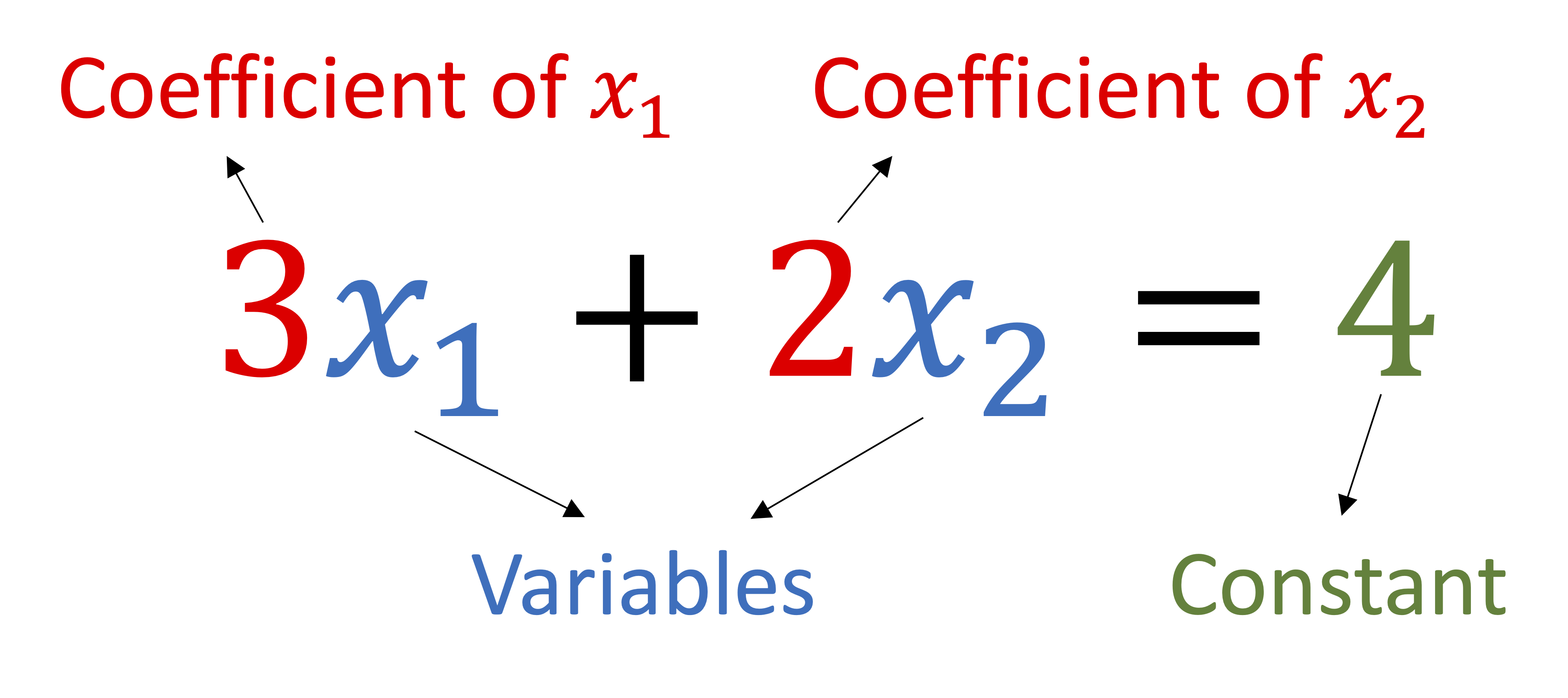
Definition 1.1.1. Linear equations.
A linear equation in the \(n\) variables \(x_1, x_2, \cdots, x_n \) is an equation that can be written in the form
where the coefficients \(a_1, a_2,\cdots, a_n \) and the independent variable \(b\) are constants.
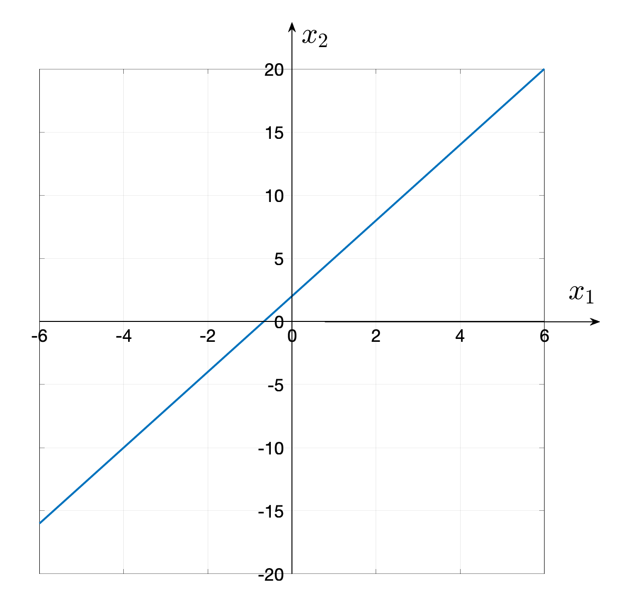
Example 1.1.2. Linear equations in 2D.
The equation of the line \(y = 3x + 2 \) can be written as
Example 1.1.3. Linear equations in 3D.
The equation of a plane is also considered a linear equation. For example
Checkpoint 1.1.4. Identify linear equations.
Determine if the given equation is linear (input y or n).
-
Is \(x = 3y - 2\) Linear?
-
Is \(y + \sin(x) = 3\) Linear?
-
Is \(a + b - 3c = 4\) Linear?
-
Is \(x_1 - x_3+ x_5 = 0\) Linear?
-
Is \(x_1^2 + x_2 = 3\) Linear?
\(\,\)
\(\text{Yes}\)
\(\text{No}\)
\(\text{Yes}\)
\(\text{Yes}\)
\(\text{No}\)
1, 3 and 4 are linear. 2 and 5 are non-linear.
The name of the variable does not matter (see 1, 3 and 4) as long as the variables are in linear form the equation is consider linear. The second equation is not linear because the trigonometric function and the last equation is not linear because the first variable is squared.
\(\, \)
Definition 1.1.5. Standard form.
In the standard form of a linear equation all terms containing unknowns are placed in the left-hand-side of the equation and all constant terms in the right-hand-side.
Example 1.1.6. Some linear equations in standard form.
-
\begin{equation*} 3x_1 - x_2 + x_3 = 2 \end{equation*}
-
\begin{equation*} a_1 x_1 + a_2 x_2 + a_3 x_3 + \cdots + a_n x_n = b \end{equation*}
\(\, \)
Definition 1.1.7. Solutions of linear equations.
A point that satisfies a linear equation is considered a solution to that equation.
Checkpoint 1.1.8. Solutions of linear equations in 2D.
Consider the equation \(3x_1 + 4x_2 = 21. \)
-
Is the point \(\left(3, -2 \right)\) a solution to this equation?
-
Is the point \(\left(0, 2 \right)\) a solution to this equation?
-
Is the point \(\left(3, 3 \right)\) a solution to this equation?
-
Is the point \(\left(7, 0 \right)\) a solution to this equation?
\(\,\)
\(\text{No}\)
\(\text{No}\)
\(\text{Yes}\)
\(\text{Yes}\)
Substitute the first coordinate for the first variable \(\left(x_1\right)\) and the second coordinate for the second variable \(\left(x_2\right)\) and if the result is \(21\) then the point is a solution to the linear equation.
Checkpoint 1.1.9. Solutions of linear equations in higher dimension.
Consider the equation \(x_1 - 4x_2 + 3x_3 - 2x_4 = -1. \)
\(\, \)
Definition 1.1.10. Systems of linear equations.
A system of linear equations consist of two or more linear equations such that all equations in the system are considered simultaneously.
The system of linear equations below consists of \(m\) equations of \(n \) variables,
Here the \(x_i\)'s are the \(\textit{unknowns}\text{,}\) the \(a_{i j}\)'s are the \(\textit{coefficients}\text{,}\) and the \(b_i\)'s are the \(\textit{independent variables}\) or right-hand-side.
Definition 1.1.11. Homogeneous systems of linear equations.
A system of equations is called homogeneous if each equation in the system is equal to 0. A homogeneous system has the form
Definition 1.1.12. Solutions to systems of linear equations.
A solution to a system of linear equations are the points that satisfy all equations in the linear system at the same time.
Example 1.1.13. Graphic solutions in 2D - case 1.
Consider the system of equations
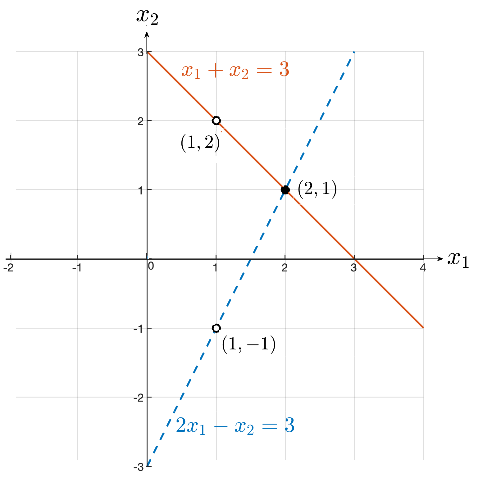
A solution to the first equation would be \(x_1 = 1, x_2 = 2 \) since
However, this is not a solution to the second equation, since
Similarly, \(x_1 = 1, x_2 =-1 \) is a solution to the second equation but not to the first. Check!
Then, according to our definition neither set of values is a solution to the system of equations.
A solution to the system of equations is \(x_1 = 2, x_2 = 1 \text{,}\) since
In this case the system has a unique solution.
Checkpoint 1.1.14. Graphic solutions in 2D - case 2.
Consider the system of linear equations depicted in the figure below.
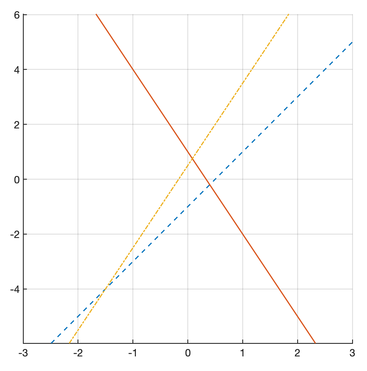
Does the system have unique solution, infinitely many solutions, or no solution?
-
Unique solution
-
Infinitely many solutions
-
No solution
\(\,\)
Checkpoint 1.1.15. Graphic solutions in 2D - case 3.
Consider the system of linear equations depicted in the figure below.
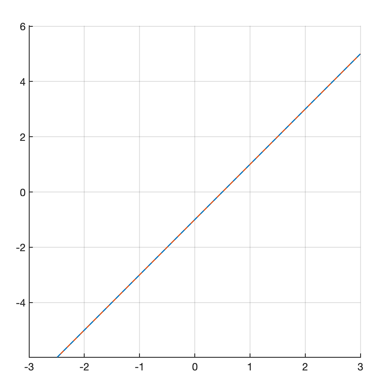
Does the system have unique solution, infinitely many solutions, or no solution?
-
Unique solution
-
Infinitely many solutions
-
No solution
\(\,\)
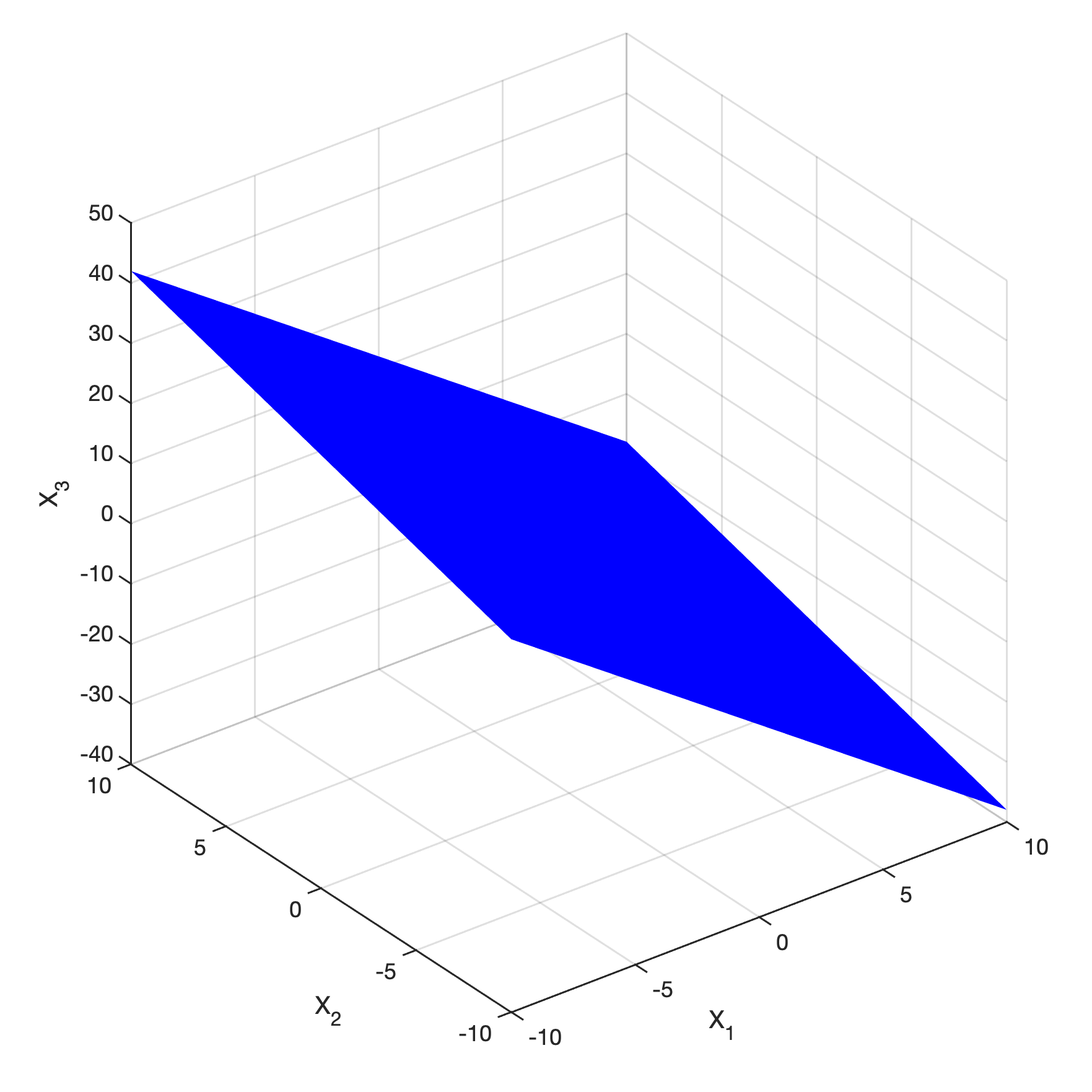
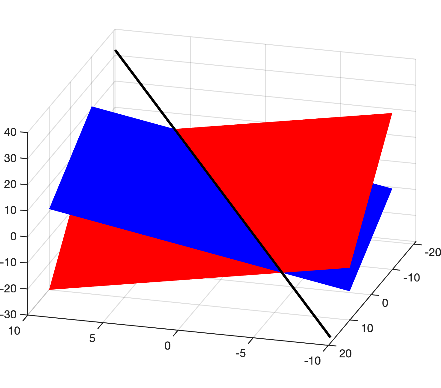
Checkpoint 1.1.16. Graphic solutions in 3D.
In previous problems we saw that, in two dimensions, solving a system of linear equations is equivalent to finding the intersection of all the lines within the system. We also know that linear equations in three dimensions correspond to planes. Using what you learned in previous problems and examples, can you determine whether the system depicted below has a unique solution, no solution or infinitely many solutions?
\(\, \)
Definition 1.1.17. Consistent systems of linear equations.
A system of linear equations is called consistent if there exists at least one solution. It is called inconsistent if there is no solution.
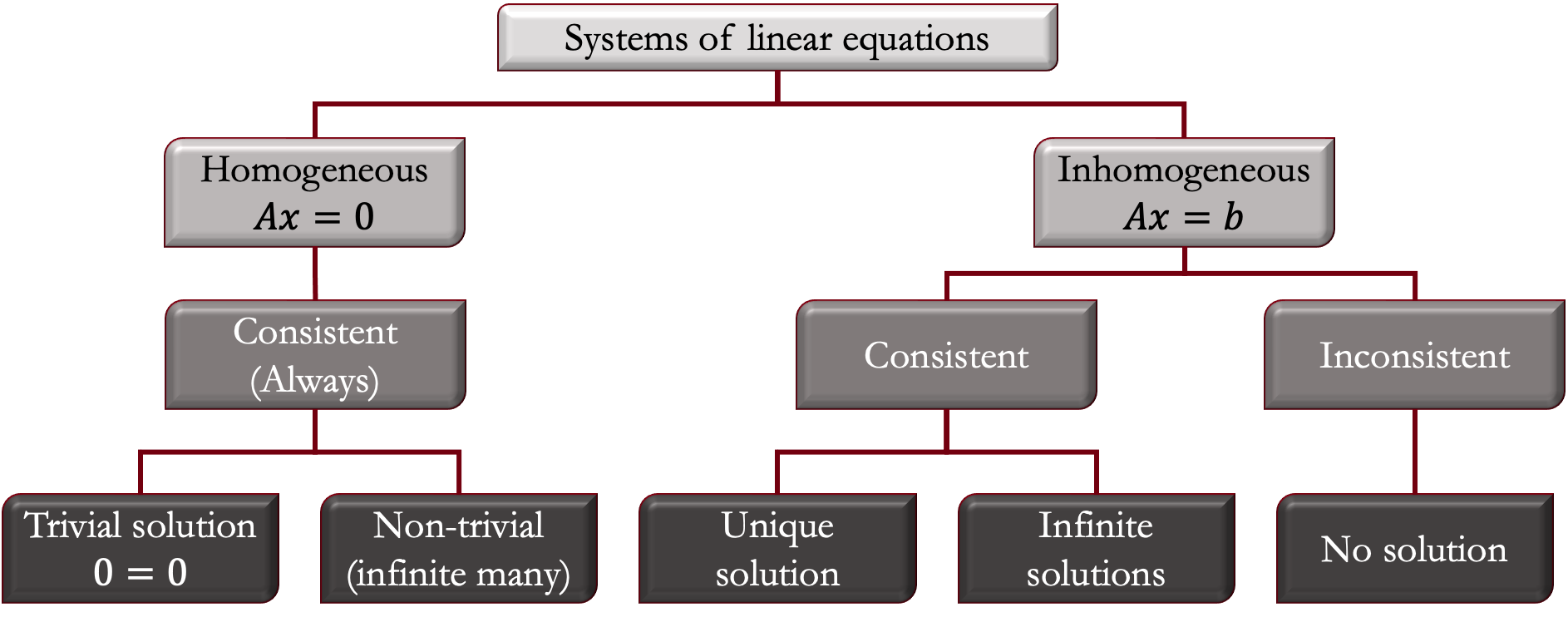
Insight 1.1.18. Summary of classification of systems of linear equations.
Subsection 1.1.2 Matrices
In linear algebra we are interested in solving linear systems of equations, however, the geometric approach used in the last section becomes cumbersome for systems with more than 3 variables, which is often the case in applications. Matrices offer an alternative for manipulating large systems of linear equations in a concise way.
Definition 1.1.19. Matrix.
A matrix is an array of numbers organized in rows and columns.
For now we are only interested in matrices
as representations of systems of linear equations. We
will come back to matrices properties and operations in
[cross-reference


                  to target(s) "chapter2" missing or not unique]
.
Subsection 1.1.3 Matrix representation of systems of linear equations
A system of linear equations can be represented in matrix form using its coefficient matrix (Subsubsection 1.1.3.1), a variable vector (Subsubsection 1.1.3.2), and a constant vector (Subsubsection 1.1.3.3).
Insight 1.1.20. Video summary.
\(\, \)
Subsubsection 1.1.3.1 Coefficient matrix
The coefficient matrix of a system of linear equations contains all the coefficients in the system of equations. In this matrix representation the rows of the matrix correspond to each equation in the system and the columns to each variable. For a system with \(m \) equations and \(n \) variables the size of the coefficient matrix is \(m \times n \text{.}\)
Example 1.1.21. Finding the coefficient matrix of a system of equations.
The system of linear equations
has the coefficient matrix:
Checkpoint 1.1.22. Finding the coefficient matrix.
Find the coefficient matrix for the given system of equations,
| \(\,\) | \(\lceil\) | \(\rceil\) | |||
| \(\boldsymbol{A} =\) | \(\vert\) | \(\vert\) | |||
| \(\,\) | \(\lfloor\) | \(\rfloor\) | |||
| \(\,\) | \(\,\) | \(\,\) | \(\,\) |
\(\, \)
Subsubsection 1.1.3.2 Variable vector
For a system with \(m \) equations and \(n \) variables the variable vector is a \(1 \times n \) matrix containing the unknowns of the system.
Example 1.1.23. Finding the variable vector of a system of equations.
The system of linear equations
has the variable vector:
\(\, \)
Subsubsection 1.1.3.3 Constant vector
When a system of linear equations is written in standard form (Definition 1.1.5) the constant vector contains the right-hand-side of the equations. For a system with \(m \) equations and \(n \) variables the constant vector is a \(1 \times m \) matrix.
Example 1.1.24. Finding the constant vector of a system of equations.
The system of linear equations
has the constant vector:
Checkpoint 1.1.25. Finding matrix representation of a system.
Consider the following system of equations,
The coefficient matrix for the system is
| \(\,\) | \(\lceil\) | \(\rceil\) | |||
| \(A =\) | \(\vert\) | \(\vert\) | |||
| \(\,\) | \(\lfloor\) | \(\rfloor\) | |||
| \(\,\) | \(\,\) | \(\,\) | \(\,\) |
The vector of variables is
| \(\,\) | \(\lceil\) | \(\rceil\) | |
| \(x =\) | \(\vert\) | \(\vert\) | |
| \(\,\) | \(\lfloor\) | \(\rfloor\) | |
| \(\,\) | \(\,\) | \(\,\) | \(\,\) |
The constant vector for the system is
| \(\,\) | \(\lceil\) | \(\rceil\) | |
| \(b =\) | \(\vert\) | \(\vert\) | |
| \(\,\) | \(\lfloor\) | \(\rfloor\) | |
| \(\,\) | \(\,\) | \(\,\) | \(\,\) |
\(\,\)
\(\, \)
Subsubsection 1.1.3.4 Augmented matrix
A system of equations can be abbreviated using a augmented matrix. To obtain the augmented matrix for a system we combine the coefficient matrix and the constant vector.
Example 1.1.26. Finding the augmented matrix of a system.
The system of linear equations
has the augmented matrix:
Note: sometimes a bar is added to the augmented matrix to differentiate the coefficient matrix from the independent vector.
Checkpoint 1.1.27. Find the augmented matrix.
Find the augmented matrix for the system of linear equations,
| \(\,\) | \(\lceil\) | \(\rceil\) | ||||
| \(\boldsymbol{A} =\) | \(\vert\) | \(\vert\) | ||||
| \(\,\) | \(\lfloor\) | \(\rfloor\) | ||||
| \(\,\) | \(\,\) | \(\,\) | \(\,\) |
\(9\)
\(-9\)
\(5\)
\(-5\)
\(4\)
\(7\)
\(-3\)
\(-4\)
\(-6\)
\(1\)
\(6\)
\(-8\)
Checkpoint 1.1.28. Find the system corresponding to a given augmented matrix.
Convert the augmented matrix
to the equivalent linear system. Use x1 and x2 to enter the variables \(x_1\) and \(x_2 \text{.}\)
=
=
=
\(\,\)
Checkpoint 1.1.29. Determine when a system is consistent.
Determine the value of \(h \) such that the matrix is the augmented matrix of a consistent linear system.
\(\,\)
\(h =\)
\(\,\)
\(\frac{-3}{2}\)
The system of equations corresponding to the augmented matrix is
From the second equation
Substituing into the first equation gives
Simplifying
Subsection 1.1.4 Homework
Link to webwork: HW 1.1