Section 1.1 Gauss-Jordan Elimination
Objectives
-
Differentiate dependent and independent systems of linear equations and classify them according to the RREF of their augmented matrix.
-
Use Gauss-Jordan elimination to solve a system of linear equations.
\(\, \)
\(\Large{\textbf{Section Content}} \)
\(\, \)
Subsection 1.1.1 Dependent and independent systems
Definition 1.1.1. Dependent system of linear equations.
A dependent system of equations has infinitely many solutions. This is characterized by having one or more free variables.
Definition 1.1.2. Independent system of linear equations.
An independent system of equations has a unique solution.
Insight 1.1.3. Updated summary of classification of systems of linear equations.

Once we obtained the RREF of the augmented matrix of a system, we can conclude -without explicitly solving the system- whether it has no solution, infinitely many solutions or unique solution. We do this by looking at the rows and leading ones in the RREF of the augmented matrix:
-
If there is a row with all zeros except the last entry, this implies the system has no solution.

-
If the number of leading ones is less than the number of variables in the system, the system has infinitely many solutions.

-
If the number of leading ones is equal to the number of variables in the system, the system has unique solution.

Example 1.1.4. Use RREF matrix to find solution.
Given the RREF matrix, find the solution to the system of equations it represents.
Since the matrix has 5 columns, the corresponding system of equations has 4 variables (4 variables + 1 independent vector = 5). Then the system represented by the matrix is
The solution is
This system has infinetely many solutions since both \(r \) and \(s \) can be any real number. We call this a dependent system.
Checkpoint 1.1.5. Dependent or independent system of equations.
Let \(\boldsymbol{A} = \begin{array}{lrrrrrr} \lceil \amp 1 \amp 0 \amp {-1} \amp 0 \amp {5} \amp \rceil \\ \vert \amp 0 \amp 1 \amp {2} \amp 0 \amp {8} \amp \vert\\ \vert \amp 0 \amp 0 \amp 0 \amp 1 \amp {7} \amp \vert\\ \lfloor \amp 0 \amp 0 \amp 0 \amp 0 \amp 0 \amp \rfloor \end{array}\)
Is the matrix in row echelon form (REF)?
-
Yes
-
No
Is the matrix in reduced row echelon form (RREF)?
-
Yes
-
No
If this matrix were the augmented matrix for a system of linear equations, would the system be inconsistent, dependent, or independent?
-
Inconsistent
-
Dependent
-
Independent
\(\text{Yes}\)
\(\text{Yes}\)
\(\text{Dependent}\)
The corresponding system for the reduced matrix is
The solution is then,
Since \(s\) can be any real number, the system has infinitely many solutions, which means the system is dependent.
Another way to see this is by comparing the number of leading ones to the number of variables. The system has 4 variables but the augmented matrix has only 3 leading ones, this implies that there will be 1 free variable, and since that free variable can take any value, the system has infinitely many solutions.
Checkpoint 1.1.6. Solutions to systems of equations.
Without explicitly solving the system and based on the RREF of the augmented matrix of a system, determine if the system has no solution (inconsistent), unique solution (independent) or infinitely many solutions (dependent).
\(\,\)
-
Inconsistent
-
Dependent
-
Independent
\(\,\)
-
Inconsistent
-
Dependent
-
Independent
\(\,\)
-
Inconsistent
-
Dependent
-
Independent
\(\text{Dependent}\)
\(\text{Inconsistent}\)
\(\text{Independent}\)
-
For the first matrix, the system has 3 variables (4 columns in the augmented matrix) and the RREF only has 3 leading ones (last row is all zeros). This means that only two variables will be defined and the third one can be anything. The system has infinitely many solutions, which makes it a dependent system.
-
For the second matrix, the last row suggests \(0 = {4},\) which is obviously not possible. The system has no solution, which makes it an inconsistent system.
-
The system has 3 variables and there are 3 leading ones, which means each variable gets a value. The system is independent since it has unique solution \(\left( x_1 = {1}, x_2 = {3}, x_3 = {-1}\right)\text{.}\)
Subsection 1.1.2 Solving systems of equations: Gauss-Jordan method
Definition 1.1.7. Gauss-Jordan elimination.
Gauss-Jordan elimination
is used to find the solution -if it exists- of a system
of linear equations. Solutions to the system are
obtained by performing elementary
row operations ([cross-reference
to target(s) "ERO" missing or not unique]) to
the augmented matrix of the system. These operations are
applied until that matrix is in reduced
echelon form ([cross-reference
to target(s) "RREF" missing or not unique]).
Solving a system of linear equations using Gauss-Jordan elimination includes:
- Find the augmented matrix of the system
- Reduced the augmented matrix to RREF
- Determine the system of equations represented by the new RREF matrix
- Solve the system
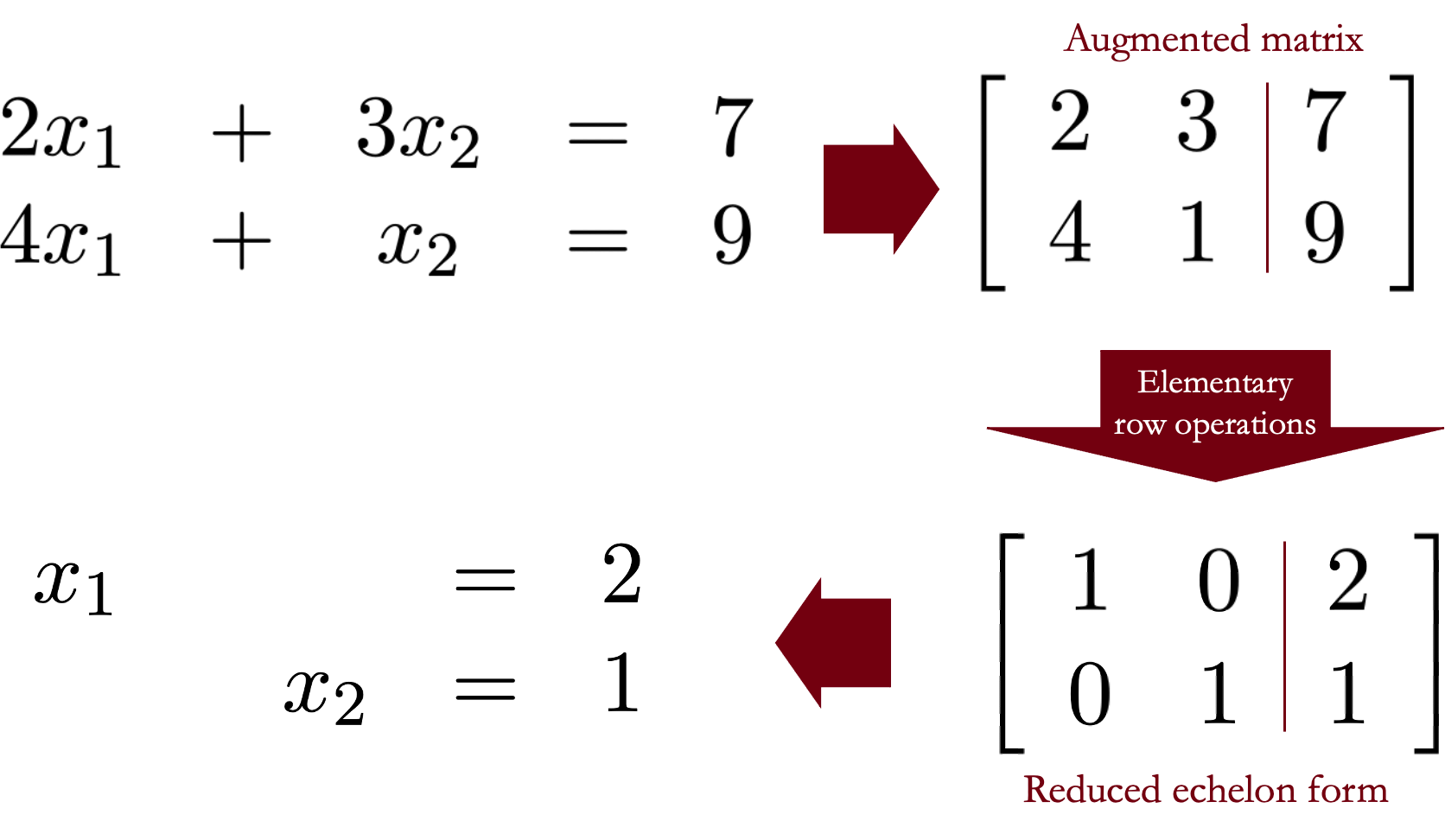
Example 1.1.8. Solving a system of equations.
Solve the following system of equations,
- Find the augmented matrix of the system
\(\hspace{0.55cm} \) 2. \(\hspace{0.03cm} \) Reduced the augmented matrix to RREF (see detailed operations in video below)
\(\hspace{0.55cm} \) 3. \(\hspace{0.03cm} \) Determine the system of equations for new RREF matrix
\(\hspace{0.55cm} \) 3. \(\hspace{0.03cm} \) Solve system
Checkpoint 1.1.9. Solve system of equations.
Use Gauss-Jordan elimination to solve the system
The reduced row echelon form of the augmented matrix is
| \(\,\) | \(\lceil\) | \(\rceil\) | ||||
| \(A_{\text{RREF}} =\) | \(\vert\) | \(\vert\) | ||||
| \(\,\) | \(\lfloor\) | \(\rfloor\) | ||||
| \(\,\) | \(\,\) | \(\,\) | \(\,\) |
The solution of the system is
| \(x_1 =\) |
| \(x_2 =\) |
| \(x_3 =\) |
\(\,\)
\(1\)
\(0\)
\(0\)
\(-2\)
\(0\)
\(1\)
\(0\)
\(-4\)
\(0\)
\(0\)
\(0\)
\(-4\)
\(-2\)
\(-4\)
\(-4\)
Subsection 1.1.3 Homework
Link to webwork: HW 1.3