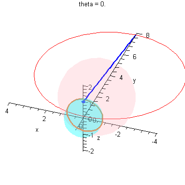
Initial Configuration: the spheres S and S_r and the point P 

>	S  := a -> x^2+(y-a)^2+z^2=a^2;  # fixed surface

 

>	Sr := r -> x^2+y^2+z^2=r^2;      # shrinking sphere

 

>	P  := r -> [ 0, 0, r ];          # top of shrinking sphere

 

>

 

>	plotP  := r -> plot3d( P(r), x=-1..1, y=-1..1, style=point, symbol=circle, symbolsize=10, color=blue ):

 

>	plotS  := a -> implicitplot3d( S(a), x= -a..a, y=0..2*a, z=-a..a,                               color=pink, style=patchnogrid, transparency=0.8 ):

 

>	plotSr := r -> implicitplot3d( Sr(r), x=-r..r, y=-r..r, z=-r..r,                          color=cyan, style=patchnogrid, transparency=0.8 ):

 

>	P1 := (r,a) -> display( [plotP(r),plotS(a),plotSr(r)],                        axes=normal, labels=["x","y","z"], orientation=[25,65] ):

 

>

P1(1,2);

 

>

 

Construction of Q: Intersection of S and S_r 

The intersection between these two spheres is a circle, parallel to the x=0 plane. 

>	Intersection := [allvalues( solve( {S(a),Sr(r)}, {x,y,z} ) )] ;

 

The two parts to this solution are the top and bottom of the circle. 

>

 

>	y1,r1 :=eval( [y, sqrt(x^2+z^2)], Intersection[1] )[]:

 

>	y2,r2 :=eval( [y, sqrt(x^2+z^2)], Intersection[2] )[]:

 

>

y1=y2;

 

>	simplify( r1=r2 ) assuming r>0, a>0;

 

>

 

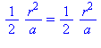
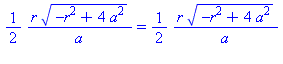
This shows that Q is the circle 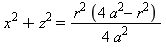   with  .  

>

 

To construct the projection from the top of the shrinking sphere through Q onto the z=0 plane, parameterize the circle Q according to the angle made the positive x axis 

>	Q := unapply( [ r1*sin(theta), y1, r1*cos(theta) ], [theta,r,a] ):

 

>

 

>	plotQ := (r,a) -> spacecurve( Q(theta,r,a), theta=0..2*Pi,                              color=gold, thickness=2 ):

 

>	P2    := (r,a) -> display( [plotP(r),plotS(a),plotSr(r),plotQ(r,a)],                           axes=normal, labels=["x","y","z"], orientation=[45,60], scaling=constrained ):

 

>	P2(1/2,2);

 

>

 

Construction of R: Projection of Q, from P, onto z=0 plane 

For each angle theta, the lines passing through P and the point Q(theta) can be parameterized in terms of the (scaled) distance measured along this line. 

>	LinePQ  := unapply( expand( (1-alpha)*P(r) + alpha*Q(theta,r,a) ), [alpha,theta,r,a] );

 

>

 

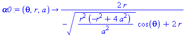
The value of the parameter alpha when these lines hit the z=0 plane are given by 

>	alpha0   := unapply( [simplify( solve( LinePQ(alpha,theta,r,a)[3]=0, alpha ) ) assuming a>0, r>0][],                     [theta,r,a] );

 

>

 

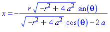
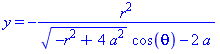
Thus, the parametric representation of of the projected curve, R, in the z=0 plane is 

>	R := unapply( [simplify( LinePQ(alpha0(theta,r,a),theta,r,a) ) assuming a>0, r>0][], [theta,r,a] );

 

>

 

This completes the constructions needed to put all of this together in one animation. 

>	plotR := (r,a) -> spacecurve( R(theta,r,a), theta=0..2*Pi, numpoints=201,                     color=red, thickness=1 ):

 

>	P3 := (r,a) -> display( [P2(r,a),plotR(r,a)] ):

 

>	animQ := (r,a) -> animate( spacecurve, [LinePQ(alpha,theta,r,a), alpha=0..alpha0(theta,r,a)], theta=0..2*Pi,                             color=blue, thickness=2, orientation=[25,65], background=P3(r,a),                             scaling=constrained, frames=41 ):

 

>	animQ(1,2);

 

>	animQ(1/2,2);

 

>

 

Limit as r -> 0 

These plots already illustrate the rapid convergence of every point on the curves R - except the one on the x-axis - to the origin (as r->0). Let's look at the parametric form of R. The three components are: 

>	X,Y,Z := R(theta,r,a)[]: x=X; y=Y; z=Z;

 

>

 

Whenever , these expression are not indeterminate (as r->0) and so 

>	map( limit, [X,Y,Z], r=0, right );

 

>

 

But, Maple misses the special case when : 

>	eval( [X,Y,Z], theta=0 );

 

>

 

The remaining limit to be evaluated is the same one that was encountered in the Shrinking Circle Problem. 

>	map( limit, , r=0, right ) assuming a>0;

 

>

 

These pointwise limits are nice, but they do no good in determining the limiting curve of the projected curves, R. 

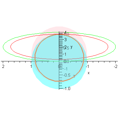
The graphical evidence suggests that the limiting curve could be a circle. If so, then the pointwise limits tell us the only possible circle will be the circle passing through both [0,0,0] and and lying in the z=0 plane. That is, 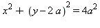, . To confirm this, the first step is to verify for each positive value of r, the projected curve R is a circle: 

>	simplify( X^2 + (Y-2*a)^2 );

 

>

 

Now, as r shrinks to zero, the square of the radius clearly increases to 

>	limit( , r=0, right );

 

>

 

We close with a different animation that shows this convergence. 

>	to3d := transform( (x,y)->[x,y,0] ):

 

>	plotR0 := a -> to3d( implicitplot( x^2 + (y-2*a)^2 = 4*a^2, x=-2*a..2*a, y=0..4*a, color=green ) ):

 

>	animR := a -> animate( P3, [1-r,a], r=0..1, frames=30, numpoints=401, paraminfo=false, background=plotR0(a) ):

 

>

animR(1);

 

>