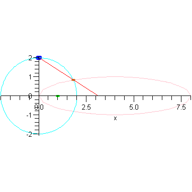
Setup the Geometry of the Problem 

>	C  := a -> ((x-a)/a)^2+y^2=1;  # fixed ellipse

 

>	Cr := r -> x^2+y^2=r^2;        # shrinking circle

 

>	P  := r -> [ 0, r ];           # top of shrinking circle

 

>

 

>	plotP  := r -> plot( [P(r)], x=-1..1, style=point, symbol=circle, symbolsize=10, thickness=3, color=blue ):

 

>	plotC  := a -> implicitplot( C(a), x= 0..2*a, y=-a..a, color=pink, grid=[25*a,25] ):

 

>	plotCr := r -> implicitplot( Cr(r), x=-r..r, y=-r..r, color=cyan ):

 

>	P1 := (r,a) -> display( [plotP(r),plotC(a),plotCr(r)], view=[-r..max(r,2*a),DEFAULT], scaling=constrained,                        axes=normal, labels=["x","y"] ):

 

>

P1(1,2);

 

>

 

The Point Q: The Intersection of C and C_r 

These ellipses intersect in two points. 

>	Intersection := [allvalues( solve( {C(a),Cr(r)}, {x,y} ) )] ;

 

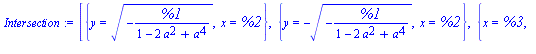
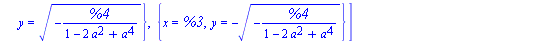
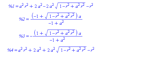
Of the two points, we want the one in the first quadrant 

>	X,Y := eval( [x,y], select( p->evalb( eval( [x,y], eval(p,[r=1.,a=2.]) )::[positive,positive] ), Intersection )[] )[]: x=X; y=Y;

 

>

 

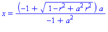
This is the formula for the point Q.  .  

>

 

To construct the projection from the top of the shrinking circle through Q onto the y=0 plane, 

>	Q := unapply( [ X, Y ], [r,a] ):

 

>

 

>	plotQ := (r,a) -> plot( [Q(r,a)], color=gold, style=point, thickness=2 ):

 

>	P2 := (r,a) -> display( [plotP(r),plotC(a),plotCr(r),plotQ(r,a)],                         axes=normal, labels=["x","y"], scaling=constrained ):

 

>

P2(1,2);

 

>

 

The Point R: The Intersection of line through PQ and the x-axis 

For each angle theta, the lines passing through P and the point Q(theta) can be parameterized in terms of the (scaled) distance measured along this line. 

>	LinePQ  := unapply( expand( (1-alpha)*P(r) + alpha*Q(r,a) ), [alpha,r,a] );

 

>

 

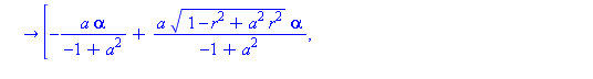
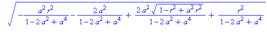
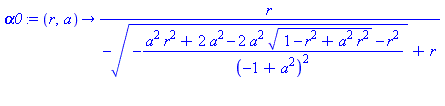
The value of the parameter alpha when these lines hit the z=0 plane are given by 

>	alpha0   := unapply( [simplify( solve( LinePQ(alpha,r,a)[2]=0, alpha ) ) assuming a>0, r>0][],                     [r,a] );

 

>

 

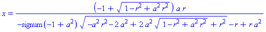
Thus, the parametric representation of of the projected point, R, in the y=0 plane is 

>	R := unapply( [simplify( LinePQ(alpha0(r,a),r,a) ) assuming a>0, r>0][], [r,a] );

 

>

 

This completes the constructions needed to put all of this together in one animation. 

>	plotR := (r,a) -> plot( [P(r),R(r,a)], color=red, thickness=1 ):

 

>	P3 := (r,a) -> display( [P2(r,a),plotR(r,a)] ):

 

>

 

These plots already illustrate the rapid convergence of every point on the curves R - except the one on the x-axis - to the origin (as r->0). Let's look at the parametric form of R. The three components are: 

>	X,Y := R(r,a)[]: x=X; y=Y;

 

>

 

The Limit as r -> 0 

Maple does not recognize the indeterminate form, initially, 

>	limit( X, r=0, right );

 

but once it is given some information about the parameter a, all is fine: 

>	limit( X, r=0, right ) assuming a>1;

 

We close with a different animation that shows this convergence. 

>	plotR0 := a -> plot( [[4/a,0]], x=0..4*a, color=green, style=point, thickness=2 ):

 

>	animR := a -> animate( P3, [2-r,a], r=0..2, frames=30, numpoints=401, paraminfo=false, background=plotR0(a), view=[-2..max(2,2*a,4/a),DEFAULT] ):

 

>

animR(4);

 

>