LemmaSS-paraboloid.mw
Shrinking Sphere Problem
Derivation of General Formula for Intersection of S and S_r,
and Its Projection from the Top of S_r onto the z=0 Plane
When S is a Paraboloid
Douglas B. Meade
9 February 2007
Initial Configuration: the S (paraboloid) and S_r (sphere) and the point P
| > |
S := (a,b,c) -> (x/a)^2-(y/b)+(z/c)^2=0; # fixed surface |
| > |
Sr := r -> x^2+y^2+z^2=r^2; # shrinking sphere |
| > |
P := r -> [ 0, 0, r ]; # top of shrinking sphere |
![(Typesetting:-mprintslash)([S := proc (a, b, c) options operator, arrow; x^2/a^2-y/b+z^2/c^2 = 0 end proc], [proc (a, b, c) options operator, arrow; x^2/a^2-y/b+z^2/c^2 = 0 end proc])](images/LemmaSS-paraboloid_1.gif)
![(Typesetting:-mprintslash)([Sr := proc (r) options operator, arrow; x^2+y^2+z^2 = r^2 end proc], [proc (r) options operator, arrow; x^2+y^2+z^2 = r^2 end proc])](images/LemmaSS-paraboloid_2.gif)
![(Typesetting:-mprintslash)([P := proc (r) options operator, arrow; [0, 0, r] end proc], [proc (r) options operator, arrow; [0, 0, r] end proc])](images/LemmaSS-paraboloid_3.gif)
| > |
plotP := r -> plot3d( P(r), x=-1..1, y=-1..1, style=point, symbol=circle, symbolsize=10, color=blue ): |
| > |
plotS := (a,b,c) -> implicitplot3d( S(a,b,c), x= -a..a, y=0..b, z=-c..c,
color=pink, style=patchnogrid, transparency=0.8, grid=[25,25,25] ): |
| > |
plotSr := r -> implicitplot3d( Sr(r), x=-r..r, y=-r..r, z=-r..r,
color=cyan, style=patchnogrid, transparency=0.8 ): |
| > |
P1 := (r,a,b,c) -> display( [plotP(r),plotS(a,b,c),plotSr(r)],
axes=normal, labels=["x","y","z"], orientation=[25,65], args[5..-1] ): |
| > |
P1(1,1,2,3, scaling=constrained); |
Construction of Q: Intersection of S and S_r
The intersection between these two solids is.
| > |
Intersection := allvalues( solve( {S(a,b,c),Sr(r)}, {x,y} ) ): |
| > |
simplify( [Intersection] ) assuming a>0, b>0, c>0; |


There are two parts to this solution.
| > |
xPOS := (p,q)->evalb( eval(x, eval(p,[r=1.,a=1.,b=1/2.,c=2.,z=1/2.]))>0 ) = q: |
| > |
Q := [ unapply( eval( [x,y,z], select( xPOS, [Intersection], true )[] ), [z,r,a,b,c] ), |
| > |
unapply( eval( [x,y,z], select( xPOS, [Intersection], false )[] ), [z,r,a,b,c] ) ]: |
| > |
piecewise( x>0, Q[1](y,r,a,b,c), x<0, Q[2](y,r,a,b,c) ); |
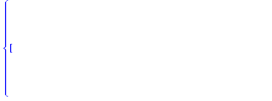


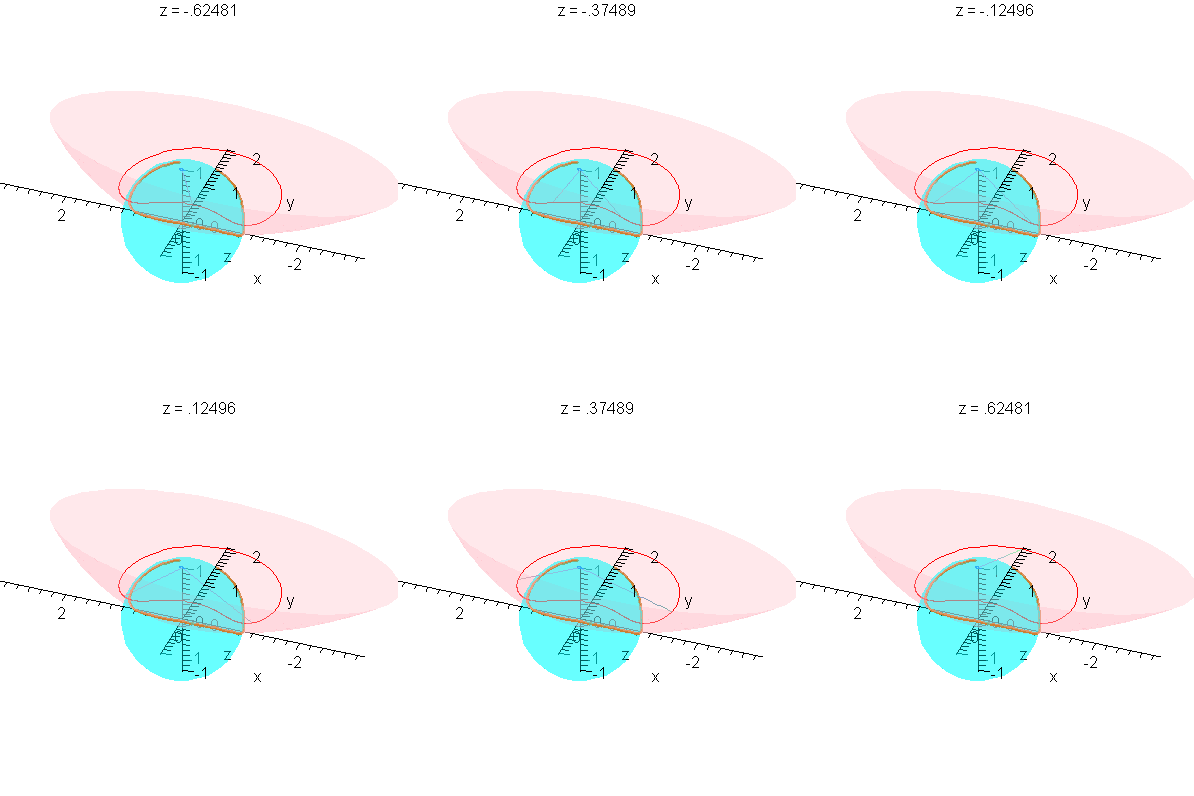
To construct the projection from the top of the shrinking sphere through Q onto the z=0 plane, the parameterization of Q can be done in terms of z. The minimum and maximum values of z occur when x=0. We now find the highest point, which we call Qstar.
| > |
yzPOS := (p,q) -> evalb( eval([y,z], eval(p,[r=1.,a=1.,b=1.,c=2.]))::[positive,positive] ) = q: |
| > |
Q0 := allvalues( solve( eval({S(a,b,c),Sr(r)},x=0), {y,z} ) ): |
| > |
Qstar := unapply( eval( [0,y,z], select( yzPOS, [Q0], true )[] ), [r,a,b,c] ): |
| > |
yM := unapply( Qstar(r,a,b,c)[2], [r,a,b,c] ); |
| > |
zM := unapply( Qstar(r,a,b,c)[3], [r,a,b,c] ); |
![(Typesetting:-mprintslash)([yM := proc (r, a, b, c) options operator, arrow; 1/4*(-2*c^2+2*(c^4+4*b^2*r^2)^(1/2))/b end proc], [proc (r, a, b, c) options operator, arrow; 1/4*(-2*c^2+2*(c^4+4*b^2*r^2)...](images/LemmaSS-paraboloid_27.gif)
![(Typesetting:-mprintslash)([zM := proc (r, a, b, c) options operator, arrow; 1/2*(-2*c^2+2*(c^4+4*b^2*r^2)^(1/2))^(1/2)*c/b end proc], [proc (r, a, b, c) options operator, arrow; 1/2*(-2*c^2+2*(c^4+4*...](images/LemmaSS-paraboloid_28.gif)
This curve is not easily identified.
| > |
plotQ := (r,a,b,c) -> display( [seq( |
| > |
spacecurve( Q[i](z,r,a,b,c), z=-zM(r,a,b,c)..zM(r,a,b,c), color=gold, thickness=2 ), |
| > |
P2 := (r,a,b,c) -> display( [plotP(r),plotS(a,b,c),plotSr(r),plotQ(r,a,b,c)],
axes=normal, labels=["x","y","z"], orientation=[45,60], scaling=constrained ): |
Construction of R: Projection of Q, from P, onto z=0 plane
For each value of z, the lines passing through P and the corresponding point on Q can be parameterized in terms of the (scaled) distance measured along this line.
| > |
LinePQ := [seq( unapply( expand( (1-alpha)*P(r) + alpha*Q[i](z,r,a,b,c) ), [alpha,z,r,a,b,c] ), i=1..2 )]: |
| > |
piecewise( x>0, LinePQ[1](alpha,z,r,a,b,c), x<0, LinePQ[2](alpha,z,r,a,b,c) ); |


The value of the parameter alpha when these lines hit the z=0 plane are given by
| > |
alpha0 := unapply( [simplify( solve( LinePQ[1](alpha,z,r,a,b,c)[3]=0, alpha ) ) assuming a>0, r>0][],
[z,r,a,b] ); |
![(Typesetting:-mprintslash)([alpha0 := proc (z, r, a, b) options operator, arrow; -r/(z-r) end proc], [proc (z, r, a, b) options operator, arrow; -r/(z-r) end proc])](images/LemmaSS-paraboloid_40.gif)
Thus, the parametric representation of of the projected curve, R, in the z=0 plane is
| > |
R := [seq( unapply( LinePQ[i](alpha0(z,r,a,b,c),z,r,a,b,c), [z,r,a,b,c] ), i=1..2 )]: |
| > |
map( simplify, piecewise( x>0, R[1](z,r,a,b,c), x<0, R[2](z,r,a,b,c) ) ); |


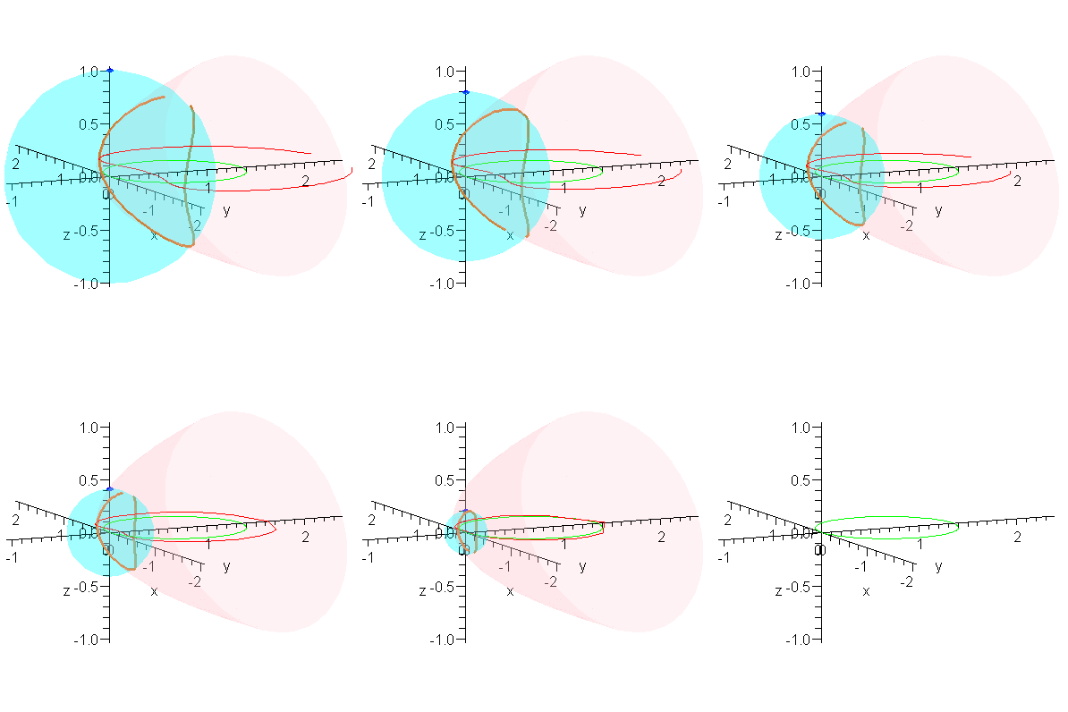
This completes the constructions needed to put all of this together in one animation.
| > |
plotR := (r,a,b,c) -> display( [seq( spacecurve( R[i](z,r,a,b,c), z=-zM(r,a,b,c).. zM(r,a,b,c), numpoints=201, color=red, thickness=1 ), i=1..2 )] ): |
| > |
P3 := (r,a,b,c) -> display( [P2(r,a,b,c),plotR(r,a,b,c)] ): |
| > |
animQ := (r,a,b,c) -> display( [seq( animate( spacecurve, [LinePQ[i](alpha,z,r,a,b,c), alpha=0..alpha0(z,r,a,b,c)], z=-zM(r,a,b,c).. zM(r,a,b,c),
color=blue, thickness=2, orientation=[25,65], background=P3(r,a,b,c),
scaling=constrained, frames=41 ), i=1..2 )] ): |
Limit as r -> 0
These plots already illustrate the rapid convergence of every point on the curves R - except the one on the x-axis - to the origin (as r->0). Let's look at the parametric form of R. The three components are (for x>0):
| > |
X,Y,Z := R[1](zeta,r,a,b,c)[]:
x=X;
y=Y;
z=Z; |


It is not surprising that Maple reports that every point converges to the origin.
| > |
map( limit, [X,Y,Z], r=0, right ); |
![[0, 0, 0]](images/LemmaSS-paraboloid_58.gif)
We know there might be something interesting happening at the highest points on Q (along the positive y-axis). These points are given by
| > |
Qstar := eval( [X,Y,Z], zeta=zM(r,a,b,c) ): |
These expressions do not simplify much, but we do see that the z-component is 0.
| > |
simplify( Qstar ) assuming a>b,b>c,c>0; |


In the limit, we expect that x approaches zero and y approaches twice the radius of the limiting circle. The general limit is still the origin
| > |
map( limit, Qstar, r=0, right ); |
![[0, 0, 0]](images/LemmaSS-paraboloid_66.gif)
but, at the highest point on Q:
| > |
map( limit, Qstar, r=0, right ) assuming a>0,b>0,c>0; |
![[0, 2*c^2/b, 0]](images/LemmaSS-paraboloid_67.gif)
This suggests that the limiting curve approached by R is the circle centered at [ 0,  , 0 ] with radius
  :
:  . Notice that the curvature of the restriction of S to the y=0 plane is
  .This result is consistent with the general conclusion (with
  =
=  ).
).
We close with an animation that shows this convergence.
| > |
to3d := transform( (x,y)->[x,y,0] ): |
| > |
plotR0 := p -> to3d( implicitplot( x^2 + (y-2*p)^2 = (2*p)^2, x=-2*p..2*p, y=0..4*p, color=green ) ): |
| > |
animR := (a,b,c) -> animate( P3, [1-r,a,b,c], r=0..1, frames=40, numpoints=401, paraminfo=false, background=plotR0(c^2/2/b) ): |
| > |
animR(2,1.5,1); # Be patient! This animation could take a while to create. |

![(Typesetting:-mprintslash)([S := proc (a, b, c) options operator, arrow; x^2/a^2-y/b+z^2/c^2 = 0 end proc], [proc (a, b, c) options operator, arrow; x^2/a^2-y/b+z^2/c^2 = 0 end proc])](images/LemmaSS-paraboloid_1.gif)
![]()
![]()


![(Typesetting:-mprintslash)([yM := proc (r, a, b, c) options operator, arrow; 1/4*(-2*c^2+2*(c^4+4*b^2*r^2)^(1/2))/b end proc], [proc (r, a, b, c) options operator, arrow; 1/4*(-2*c^2+2*(c^4+4*b^2*r^2)...](images/LemmaSS-paraboloid_27.gif)
![(Typesetting:-mprintslash)([zM := proc (r, a, b, c) options operator, arrow; 1/2*(-2*c^2+2*(c^4+4*b^2*r^2)^(1/2))^(1/2)*c/b end proc], [proc (r, a, b, c) options operator, arrow; 1/2*(-2*c^2+2*(c^4+4*...](images/LemmaSS-paraboloid_28.gif)


![(Typesetting:-mprintslash)([alpha0 := proc (z, r, a, b) options operator, arrow; -r/(z-r) end proc], [proc (z, r, a, b) options operator, arrow; -r/(z-r) end proc])](images/LemmaSS-paraboloid_40.gif)


![[0, 2*c^2/b, 0]](images/LemmaSS-paraboloid_67.gif)
 . Notice that the curvature of the restriction of S to the y=0 plane is
  .This result is consistent with the general conclusion (with
  =
= 