Area.html

Area of a Plane Region

> restart;
with( plots ):

Warning, the name changecoords has been redefined

>

Lesson Overview

Area is used in the Riemann Sums lesson to begin the development of the Definite Integral. In that context all areas are computed as explicit limits. The Fundamental Theorems of Calculus and Evaluating Definite Integrals lessons provide efficient tools for the evaluating a definite integral. The essential idea developed in this lesson is summarized as

slice, approximate, limit, evaluate.

This is the general process used to express the area of a plane region as a definite integral and evaluate the integral. This same process is used in the other applications considered in this unit --- Volume of a Solid, Length of a Plane Curve, and Work --- as well as many other applications of the definite integral.

Maplet Request: Area

It would be nice to have an Area maplet. This maplet would allow the user to indicate if the region is vertically or horizontally simple. For vertically simple regions, the top and bottom would be entered as y=(function) and the endpoints would be x=(number). For horizontally simple regions, the left and right would be x=(function) and the endpoints would be y=(number). Visually, it would be ideal to have a slider located under (vert. simple) or to the left (horiz. simple) of the plot of the region. As the slider moves, the corresponding slice of the area would be highlighted. (I am thinking that the region would be filled.) If the slider idea is too difficult or not possible, then I would like to show the slices as an animation. The number of frames could be entered by the user (a slider for the # of frames would prevent users from entering too many frames).

>

Example 1: Region Between Two Curves

The region bounded by the graphs of

> top1 := sqrt(x):
y = top1;

and

> bot1 := x^2:
y = bot1;

on the interval [ 0, 1 ] is shown in the following plot

> plot( [top1,bot1], x=0..1, color=[red,blue], legend=["top: y=sqrt(x)","bottom: y=x^2"] );

>

The area of this region is given by the definite integral

> A1 := Int( top1-bot1, x=0..1 ):
Area = A1;
`` = value( A1 );

>

Example 2: Positive and Negative Area

The area between the graphs of

> f2 := sqrt(x):
y = f2;

and

> g2 := exp(-3*x):
y = g2;

on the interval [ 0, 1 ] consists of two parts, as shown in the following plot.

> P0 := plot( [[1,exp(-3)],[1,1]], color=green, legend=["x = 1"] ):
P1 := plot( [f2,g2], x=0..1, color=[red,blue], legend=["y = sqrt(x)", "y = exp(-3*x)"] ):
display( [P1,P0] );

The first piece of the area has the exponential curve as the upper boundary and the square root as the lower boundary; after the curves intersect, these roles are reversed. The following plot emphasizes this

> P2 := plot( [ max(f2,g2), min(f2,g2) ], x=0..1, color=[yellow,cyan], legend=["Top", "Bottom"], thickness=5 ):
display( [ P1, P2, P0] );

>

The definite integral for the total area enclosed

> A1 := Int( g2-f2, x=0..T ):
A2 := Int( f2-g2, x=T..1 ):
Area = A1 + A2;

where is the -coordinate of the point where the two curves intersect:

> T_exact := solve( f2=g2, x ):
T_approx := evalf( T_exact ):
T = T_exact;
`` = T_approx;

> Area = A1 + A2;
`` = value( eval( A1 + A2, T=T_approx ) );

>

Example 3: Horizontal Slices

The region bounded by the horizontal line ,

> y = f2;

and

> y = g2;

lies above the graph of for x in [ 0, ] and above the graph of for x in [ , 1 ]. That is, using vertical slices, the area can be represented as

> A_v := Int( 1-g2, x=0..T ) + Int( 1-f2, x=T..1 ):
Area = A_v;
`` = value( eval( A_v, T=T_approx ) );

>

This area can be represented as a single definite integral if horizontal slices are used. To work with horizontal slices requires writing the left and right boundaries as functions of . The left boundary is formed by the graph of , or

> left3 := solve( y=f2, x ):
x = left3;

The right boundary is formed by the graph of , or

> right3 := solve( y=g2, x ):
x = right3;

Let denote the y-coordinate of the intersection point of the two graphs:

> S_exact := simplify( eval( g2, x=T_exact ) ):
S_approx := evalf( S_exact ):
S = S_exact;
`` = S_approx;

Note that this value could also be obtained by solving the equation

> q1 := left3 = right3:
q1;

for :

> q2 := solve( q1, y ):
q2 = simplify( q2 );

The region with the left, right, and top boundaries highlighted is

> P3 := implicitplot( x=left3, x=0..1, y = S_approx..1, color=yellow, legend="Left", thickness=5 ):
P4 := implicitplot( x=right3, x=0..1, y = S_approx..1, color=cyan, legend="Right", thickness=5 ):
P5 := plot( 1, x=0..1, color=coral, legend="Top", thickness=5 ):
display( [ P1, P3, P4, P5 ] );

>

The area of this region can now be written as a single definite integral:

> A_h := Int( left3-right3, y=S..1 ):
Area = A_h;
`` = value( eval( A_h, S=S_approx ) );

Fortunately, the two different approaches to finding the area of this region agree!

>

Example 4: Area of an Ellipse

The area of an ellipse with axes of length a and b is the area of region bounded by the graph of

> q3 := (x/a)^2 + (y/b)^2 = 1:
q3;

> P6 := implicitplot( eval(q3,[a=1,b=2]), x=-3..3, y=-3..3, scaling=constrained, numpoints=1000, tickmarks=[0,0] ):
P7 := textplot( [ [1/2,0.05,"a"], [0.05,1,"b"] ], font=[TIMES,ITALIC,15], align={ABOVE,RIGHT} ):
display( [ P6, P7 ] );

>

> top4 := solve( q3, y )[1];

> right4 := solve( q3, x )[1];

>

> A_ell_v := 4 * Int( top4, x=0..a ):
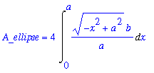
A_ellipse = A_ell_v;

While this integral cannot be evaluated using the integration techniques discussed in this course, it can be evaluated. The key is to factor the b/a out of the integal and to observe that the remaining definite integral

> q4 := Int( sqrt( a^2-x^2 ), x=0..a ):
q4;

is one fourth of the area of a circle with radius a. That is,

> q4 = value( q4 ) assuming a>0;

As a result, the area of an ellipse with radii a and b is = 4 ( ) = :

>

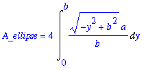
Note that this formula does reduce to the area of a circle with radius when . Note also that this result could have been obtained with horizontal slices. The definite integral for that scenario is

> A_ell_h := 4 * Int( right4, y=0..b ):
A_ellipse = A_ell_h;

Evaluation of this integral is almost identical to the one encountered with vertical slices. Factor out , recognize the remaining integral as one-fourth of the area of a circle with radius , then simplify to obtain:

> A_ellipse = A_ell_h;
`` = value( A_ell_h ) assuming a>0, b>0;

As expected, the two different slicing methods lead to the same answer.

>

Lesson Summary

The computation of areas is one of the fundamental applications of the definite integral. A definite integral for the area of a plane region can be found by adding up an appropriate collection of infinitely thin horizontal or vertical slices. The integrand is the length of each slice and the limits of integration correspond to the smallest and largest values of the independent variable that describe the region.

The area of a v ertically simple region described by

<= <= for all <= <=

The area of a horizontally simple region described by

<= <= for all <= <=

While it is important to be able to evaluate a definite integral for an area, the step that requires real skill and understanding is coming up with the definite integral.

>

What's Next?

Prior to completing the online homework assignment, you should dedicate time to practicing setting up definite integrals for the area of a plane region. The assigned problems from the text provide additional assessment of your mastery of your ability to set up definite integrals for areas.

The next lesson in this unit considers area in the graphical interpretation of the Mean Value Theorem for Integrals. In this lesson the average value of a function will be developed using the slice, approximate, limit, evaluate process. The remaining lessons in this unit, Volume of a Solid, Length of a Plane Curve, and Work, use the same general process to develop additional geometric and physical properties.

>