PLOT_TO_PS
PostScript Graphics Creation

PLOT_TO_PS is a FORTRAN90 program which reads a text file of plot commands and creates a PostScript file.

I often use this utility to make simple graphics illustrations.

Commands:

ARC X Y R ANGLE1 ANGLE2

draw the circular arc from ANGLE1 to ANGLE2, for a circle of radius R and center (X,Y).

ARROW X1 Y1 X2 Y2

draw an arrow from (X1,Y1) to (X2,Y2).

CIRCLE X Y R

draw a circle of radius R and center (X,Y).

CIRCLE_FILL X Y R

draw a circle of radius R and center (X,Y) and fill it with the current fill color.

DEBUG

switch the debugging state.

DRAWTO X Y

draw a line from the current point to (X,Y).

ELLIPSE X Y R1 R2 ANGLE

draw an ellipse centered at (X,Y) with axes lengths R1 and R2, an an angle ANGLE.

ELLIPSE_FILL X Y R1 R2 ANGLE

draw an ellipse centered at (X,Y) with axes lengths R1 and R2, an an angle ANGLE, and fill it with the current color.

ENDFILE

indicate the end of the file.

ENDPAGE

indicate the end of this "page" or image.

FILE NAME

specifies the name of the output file.

FILL_GRAY GRAY

sets the fill color to the given shade of gray.

FILL_RGB R G B

sets the fill color to the given RGB color.

FONT_SIZE H

sets the font size to the given height.

GRID X1 Y1 X2 Y2 N1 N2

draws an N1 by N2 grid in the box from (X1,Y1) to (X2,Y2).

HIST_FAT W

sets the width of histogram bars to W.

HISTOGRAM (followed by X,Y pairs, then END)

processes histogram data.

LABEL text

prints the text at the current position and current font size and current line color.

LABEL_SLANT ANGLE

sets a slant angle for a label.

LINE X1 Y1 X2 Y2

draws a line from (X1,Y1) to (X2,Y2).

LINE_GRAY GRAY

sets the line color to the given gray shade.

LINE_RGB R G B

sets the line color to the given RGB color.

LINE_WIDTH N

sets the line width. 1 is the finest.

LINETO X Y

draws a line from the current point to (X,Y). Same as DRAWTO.

MOVETO X Y

moves to (X,Y) without drawing.

PAGE

begins a new page or image.

POINT X Y

draws a point at (X,Y).

POINT_LIST (followed by X,Y pairs, then END)

draws a point at each of the (X,Y) pairs that follow.

POLYGON (followed by X,Y pairs, then END)

draws a outlined polygon by connecting the (X,Y) pairs that follow.

POLYGON_FILL (followed by X,Y pairs, then END)

draws a filled polygon by connecting the (X,Y) pairs that follow.

RADIUS X Y R ANGLE

for the circle of radius R and center (X,Y), draw the radial line at angle ANGLE.

SECTOR X Y R ANGLE1 ANGLE2

draws the sector of a circle centered at (X,Y) with radius R, from ANGLE1 to ANGLE2.

SECTOR_FILL X Y R ANGLE1 ANGLE2

draws the sector of a circle centered at (X,Y) with radius R, from ANGLE1 to ANGLE2, and fills it with current color.

SPACE X1 Y1 X2 Y2

defines the coordinate space to use in the current page.

SQUARE X Y R

draws a square centered at (X,Y) with radius R.

SQUARE_FILL X Y R

draws a square centered at (X,Y) with radius R and fills it.

STAR X Y R

draws a star centered at (X,Y) with radius R.

STAR_CIRCLE X Y R

draws open circles at the ten vertices of a star centered at (X,Y) with radius R.

STAR_DISK X Y R

draws filled disks at the ten vertices of a star centered at (X,Y) with radius R.

TRIANGLE X1 Y1 X2 Y2 X3 Y3

draws a triangle with the given vertices.

TRIANGLE_FILL X1 Y1 X2 Y2 X3 Y3

draws a triangle with the given vertices, and fills it with the current color.

Licensing:

The computer code and data files described and made available on this web page are distributed under the GNU LGPL license.

Languages:

PLOT_TO_PS is available in a FORTRAN90 version

Related Data and Software:

GRF_TO_EPS, a FORTRAN90 program which converts a GRF file to EPS format;

POINTS_01_PLOT, a MATLAB program which reads an ASCII file containing points in the unit square, and makes an Encapsulated PostScript image;

PS_WRITE, a FORTRAN90 library which implements PostScript graphics routines that is used by PLOT_TO_PS.

TRIANGULATION_PLOT, a FORTRAN90 program which makes a PostScript image of a triangulation of points.

VECTOR_PLOT, a FORTRAN90 program which plots velocity fields and the velocity direction fields.

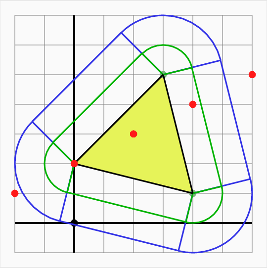
VORONOI_PLOT, a FORTRAN90 program which plots the Voronoi neighborhoods of points in the 2D unit square, using L1, L2 or LInfinity norms;

XY_DISPLAY, a MATLAB program which reads XY information defining points in 2D, and displays an image in a MATLAB graphics window;

XY_DISPLAY_OPENGL, a C++ program which reads XY information defining points in 2D, and displays an image using OpenGL.

XYL_DISPLAY, a MATLAB program which reads XYL information defining points and lines in 2D, and displays an image in a MATLAB graphics window.

XYL_DISPLAY_OPENGL, a C++ program which reads XYL information defining points and lines in 2D, and displays an image using OpenGL.

XYZ_DISPLAY, a MATLAB program which reads XYZ information defining points in 3D, and displays an image in the MATLAB graphics window.

XYZ_DISPLAY_OPENGL, a C++ program which reads XYZ information defining points in 3D, and displays an image using OpenGL.

Reference:

1. Henry McGilton, Mary Campione,
   PostScript by Example,
   Addison-Wesley,
   ISBN: 0-201-63228-4

Source Code:

• plot_to_ps.f90, the source code;

Examples and Tests:

Note that the program creates a PostScript file, but that, for display on this web page, we have used the ImageMagick program convert to convert them to PNG files.

123 is an attempt to make a plot of "1, 2, 3"

• 123.plot, the input;
• 123.png, the resulting PNG file.

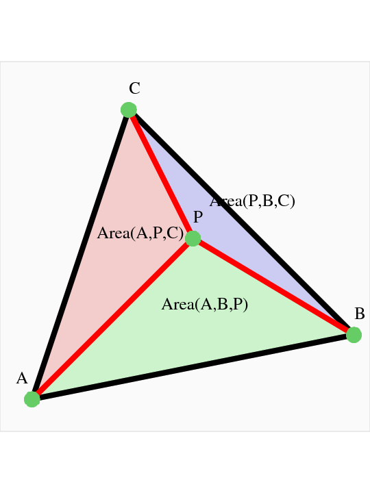
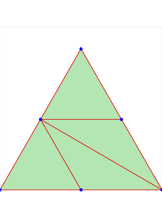
AREA_BASIS illustrates how the barycentric coordinates of a point in a triangle can be defined by the relative areas of subtriangles:

• area_basis.plot, the input;
• area_basis.png, the resulting PNG file.

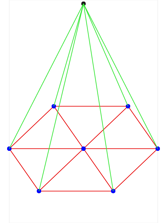
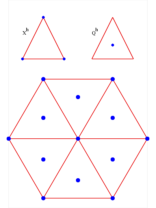
BILL_020 is a figure for page 20 of Bill's book, a plot of a typical linear basis function for a grid of triangular elements arranged in a hexagonal grid:

• bill_020.plot, the input;
• bill_020.png, the resulting PNG file.

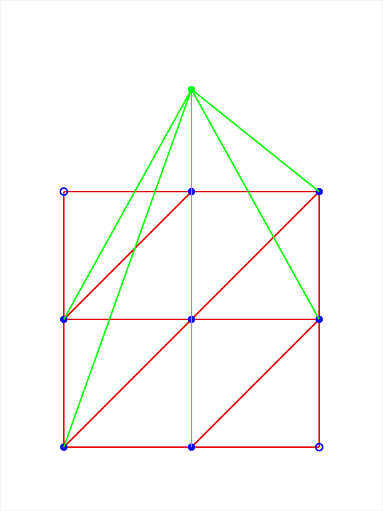
BILL_020_RECTANGLE is a version of BILL_020 in which the elements of interest are included in a rectangular grid.

• bill_020_rectangle.plot, the input;
• bill_020_rectangle.png, the resulting PNG file.

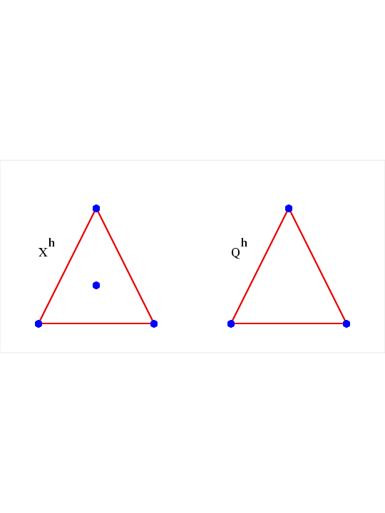
BILL_055 is a figure for page 55 of Bill's book:

• bill_055.plot, the input;
• bill_055.png, the resulting PNG file.

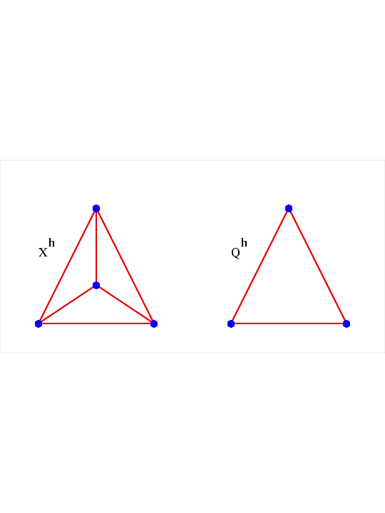
BILL_060 is a figure for page 60 of Bill's book:

• bill_060.plot, the input;
• bill_060.png, the resulting PNG file.

BILL_061 is a figure for page 61 of Bill's book:

• bill_061.plot, the input;
• bill_061.png, the resulting PNG file.

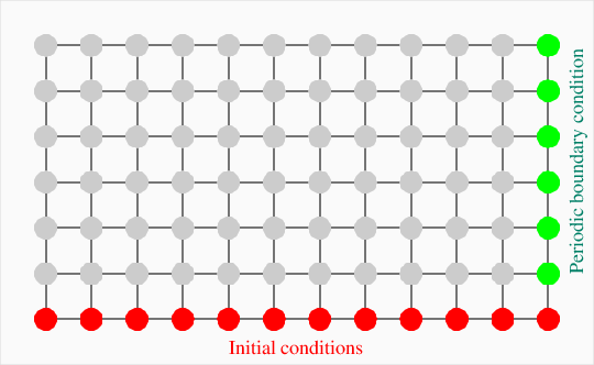
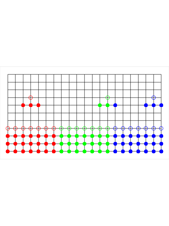
BURGERS_EQUATION is a 2D grid of points for a discretized Burgers equation, with red nodes for initial condition, green for boundaries, and gray for initially unknown:

• burgers_equation.plot, the input;
• burgers_equation.png, the resulting PNG file.

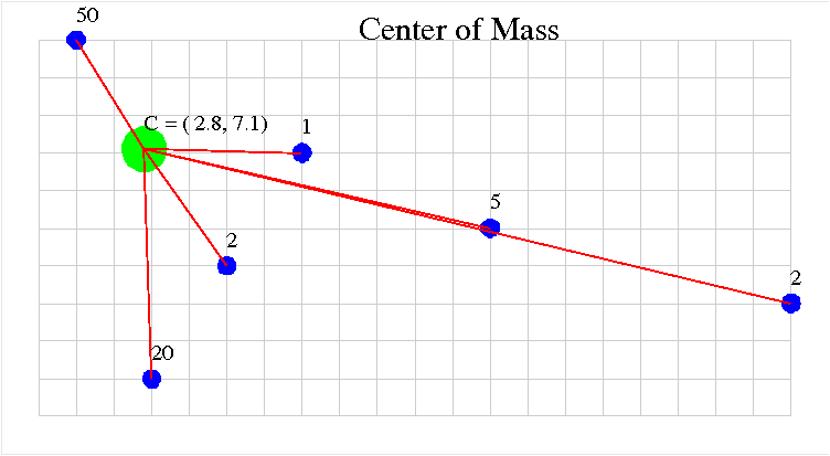
CENTER_OF_MASS plots the center of mass of 6 weighted points:

• center_of_mass.plot, the input;
• center_of_mass.png, the resulting PNG file.

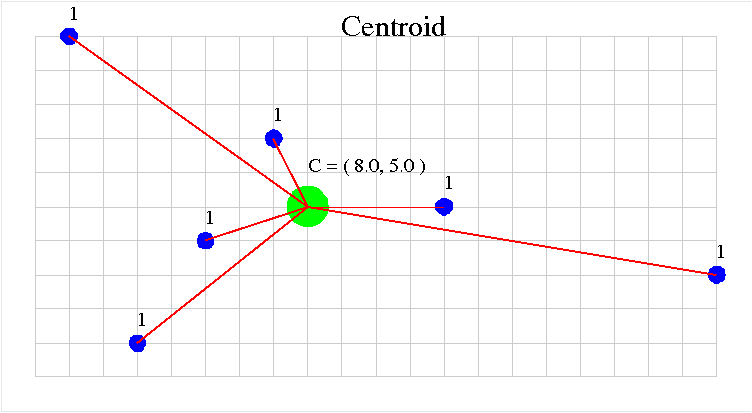
CENTROID plots the centroid of 6 (equally weighted) points:

• centroid.plot, the input;
• centroid.png, the resulting PNG file.

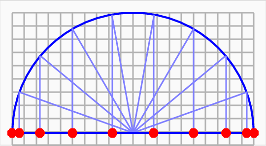
CHEBYSHEV illustrates the determination of the Chebyshev points.

• chebyshev.plot, the input;
• chebyshev.png, the resulting PNG file.

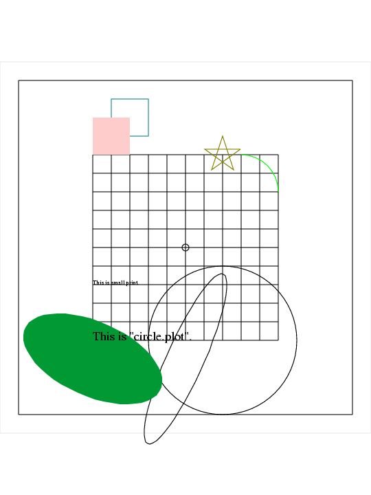
CIRCLE is a plot of a circle:

• circle.plot, the input;
• circle.png, the resulting PNG file.

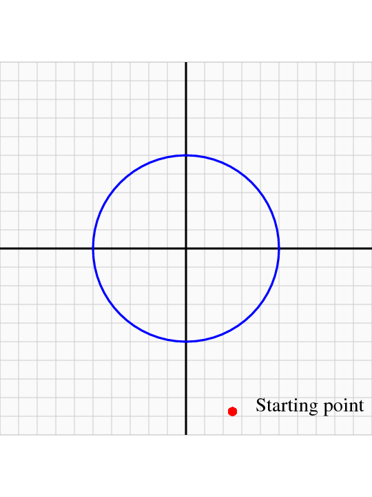
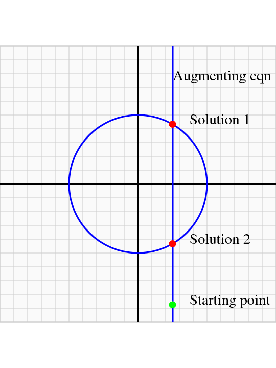
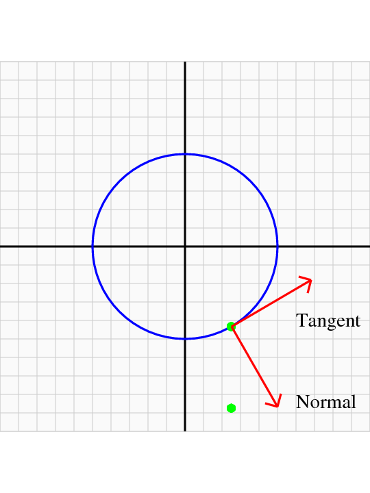
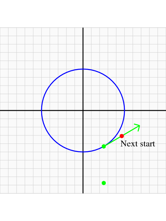
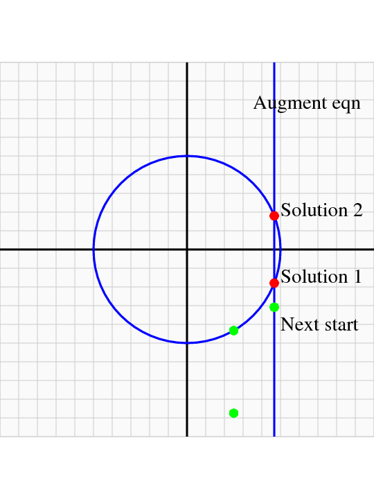
CIRCLE* illustrates a continuation process for finding successive points on a circle.

• circle1.plot, the input;
• circle1.png, the PNG file.
• circle2.plot, the input;
• circle2.png, the PNG file.
• circle3.plot, the input;
• circle3.png, the PNG file.
• circle4.plot, the input;
• circle4.png, the PNG file.
• circle5.plot, the input;
• circle5.png, the PNG file.

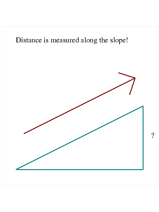
CLIMB is an illustration for a trigonometry problem, without which, our students, upon hearing that a train climbed 1 mile up a slope, would draw a diagram in which the horizontal distance was 1 mile:

• climb.plot, the input;
• climb.png, the resulting PNG file.

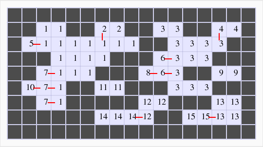
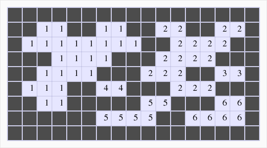
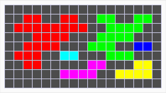
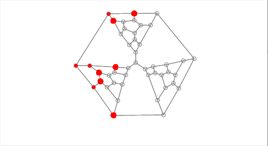
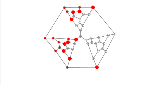
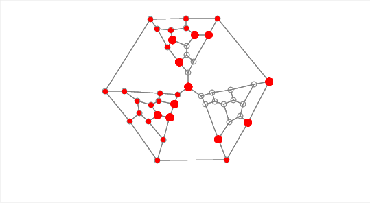
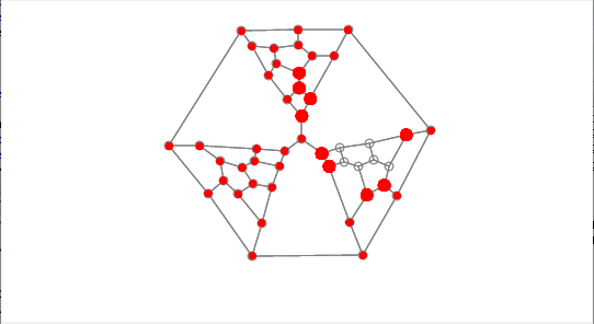
COMPONENTS_** illustrate the connected components algorithm.

• components_01.plot, the input;
• components_01.png, a PNG image.
• components_02.plot, the input;
• components_02.png, a PNG image.
• components_03.plot, the input;
• components_03.png, a PNG image.
• components_04.plot, the input;
• components_04.png, a PNG image.

CONVEX_COMBINATION illustrate two points can determine a line that is parameterized by combination coefficients that sum to 1. When the combination is "convex", the resulting point is between the two endpoints.

• convex_combination.plot, the input;
• convex_combination.png, the resulting PNG file.

CONVEX_HULL illustrate the computation of the convex hull.

• convex_hull_edge0.plot, the input;
• convex_hull_edge0.png, the resulting PNG file.
• convex_hull_edge1.plot, the input;
• convex_hull_edge1.png, the resulting PNG file.
• convex_hull_edge2.plot, the input;
• convex_hull_edge2.png, the resulting PNG file.
• convex_hull_edge3.plot, the input;
• convex_hull_edge3.png, the resulting PNG file.
• convex_hull_edge4.plot, the input;
• convex_hull_edge4.png, the resulting PNG file.
• convex_hull.plot, the input;
• convex_hull.png, the resulting PNG file.

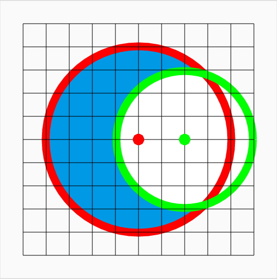
CRESCENT illustrates the construction of a crescent shape from two circles.

• crescent.plot, the input;
• crescent.png, the resulting PNG file.

DIATOM fills in a region by plotting lots of points in it:

• diatom.plot, the input;
• diatom.png, the resulting PNG file.

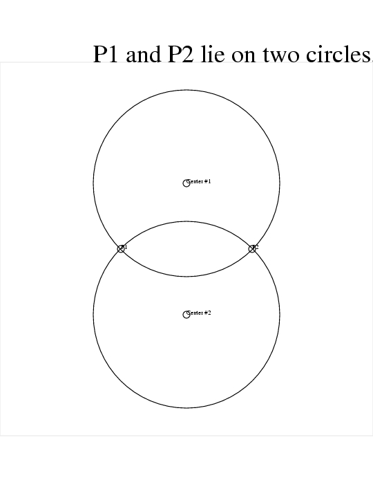
DOUBLE_CIRCLE is a plot of intersecting circles:

• double_circle.plot, the input;
• double_circle.png, the resulting PNG file.

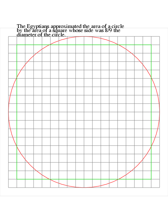
EGYPTIAN illustrates an odd fact about Egyptian mathematics:

• egyptian.plot, the input;
• egyptian.png, the resulting PNG file.

FEM_MESH_1D illustrates the construction of nodes and elements for a 1D finite element mesh:

• fem_mesh_1d.plot, the input;
• fem_mesh_1d.png, the resulting PNG file.

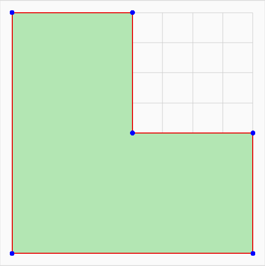
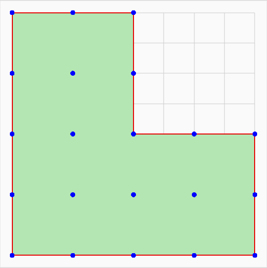
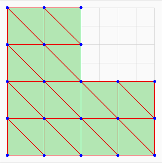
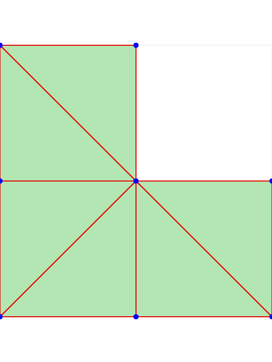
ELL illustrates the construction of nodes and elements for a 2D finite element mesh on an L-shaped region:

• ell_region.plot, the region.
• ell_region.png, the resulting PNG file.
• ell_nodes.plot, the nodes.
• ell_nodes.png, the resulting PNG file.
• ell_elements.plot, the elements.
• ell_elements.png, the resulting PNG file.

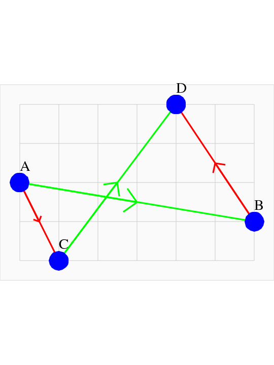
GRAPH_DIJKSTRA illustrates a graph used to demonstrate Dijkstra's shortest path algorithm.

• graph_dijkstra.plot, the input;
• graph_dijkstra.png, the resulting PNG file.

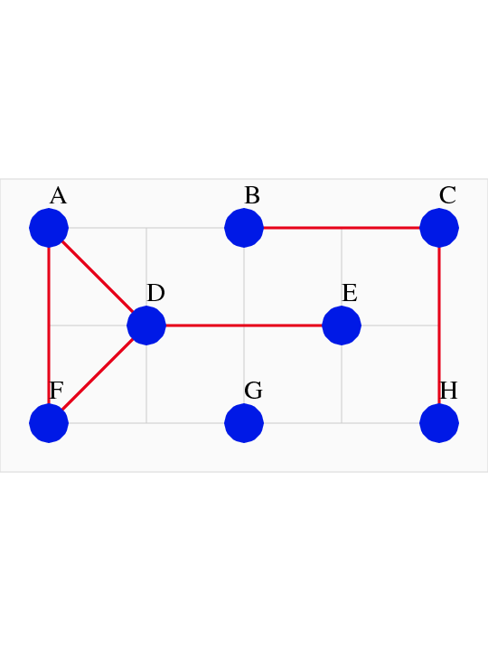
GRAPH_DISCONNECTED illustrates a disconnected graph

• graph_disconnected.plot, the input;
• graph_disconnected.png, the resulting PNG file.

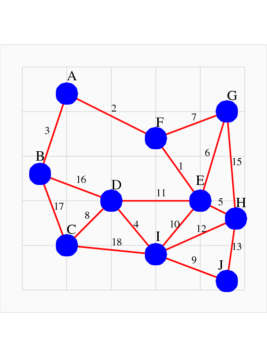
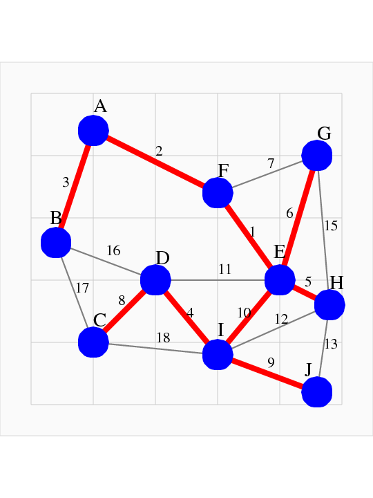
GRAPH_MST illustrates a graph suitable for the minimum spanning tree problem, with 10 nodes and 17 links labeled with lengths.

• graph_mst.plot, the input;
• graph_mst.png, the resulting PNG file.

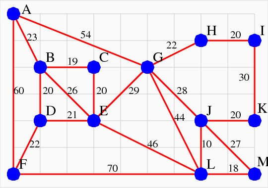
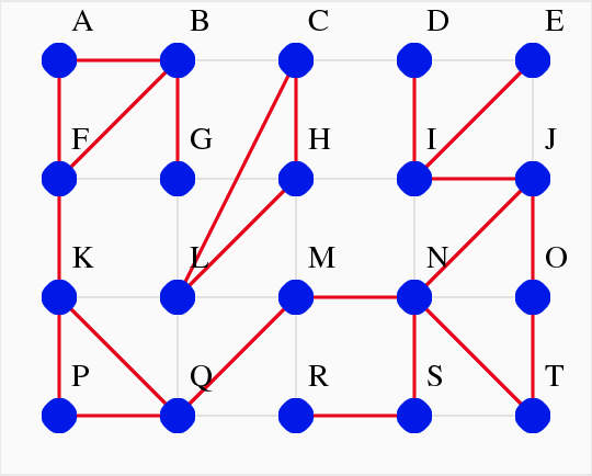
GRAPH_MST2 illustrates a graph suitable for the minimum spanning tree problem, with 13 nodes and 21 links labeled with lengths.

• graph_mst2.plot, the input;
• graph_mst2.png, the resulting PNG file.

GRAPH_MST_TREE illustrates one spanning tree for the GRAPH_MST graph.

• graph_mst_tree.plot, the input;
• graph_mst_tree.png, the resulting PNG file.

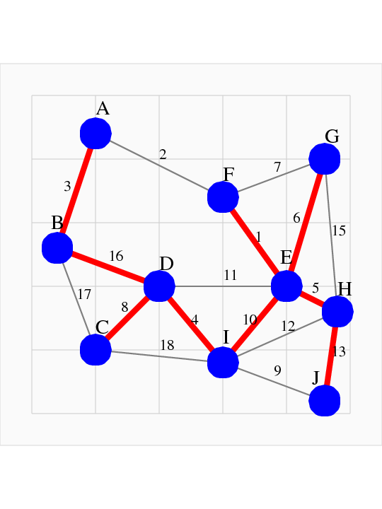
GRAPH_MST_TREE_MINIMAL illustrates the minimal spanning tree for the GRAPH_MST graph.

• graph_mst_tree_minimal.plot, the input;
• graph_mst_tree_minimal.png, the resulting PNG file.

GRAPH_PATHS is a graph on which we can ask the question of whether you can reach node A from node B.

• graph_paths.plot, the input;
• graph_paths.png, the resulting PNG file.

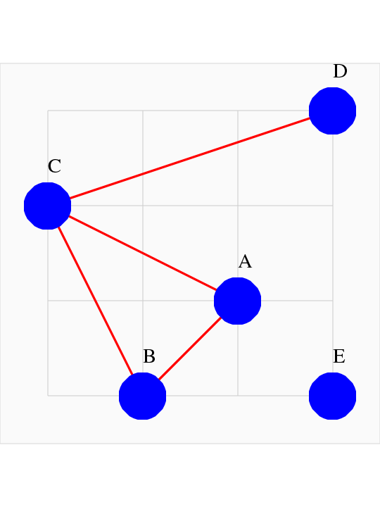
GRAPH_SIMPLE illustrates a simple graph with 5 nodes and 4 links on a 3x3 bit of graph paper.

• graph_simple.plot, the input;
• graph_simple.png, the resulting PNG file.

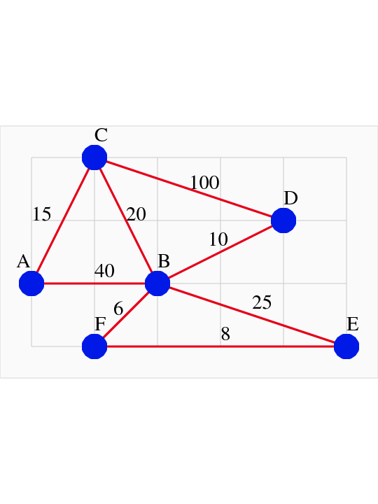
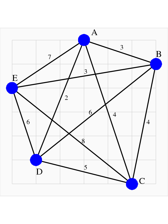
GRAPH_TSP illustrates a graph suitable for the minimum spanning tree problem or the traveling salesman problem, with 5 nodes and 10 links labeled with lengths.

• graph_tsp.plot, the input;
• graph_tsp.png, the resulting PNG file.
• graph_tsp_solution.plot, the input, displaying the solution.
• graph_tsp.png, the resulting PNG file.

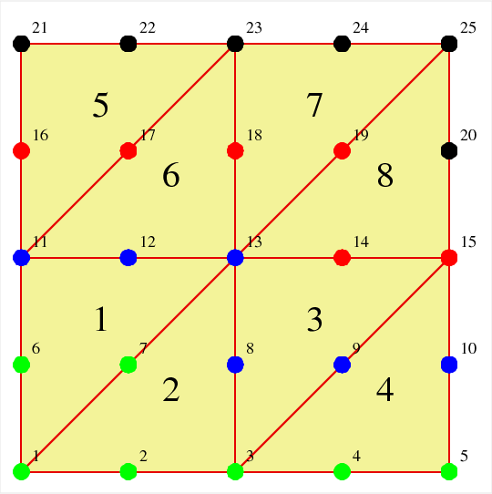
GRID_CLIFF is a small finite element grid for Gene Cliff:

• grid_cliff.plot, the input;
• grid_cliff.png, the resulting PNG file.

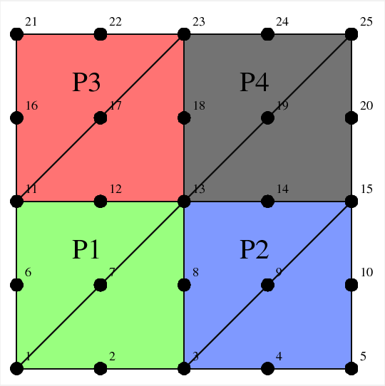
GRID_CLIFF2 illustrates how portions of the grid in GRID_CLIFF might be assigned to separate processors:

• grid_cliff2.plot, the input;
• grid_cliff2.png, the resulting PNG file.

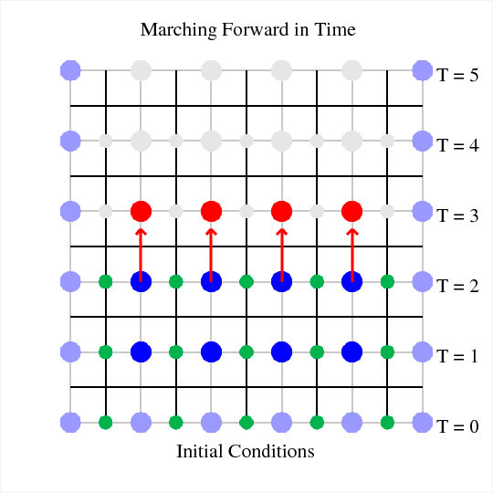
HEAT_EQUATION illustrates how a discretized version of the 1D time dependent heat equation might be set up and solved.

• heat_equation.plot, the input;
• heat_equation.png, the resulting PNG file.

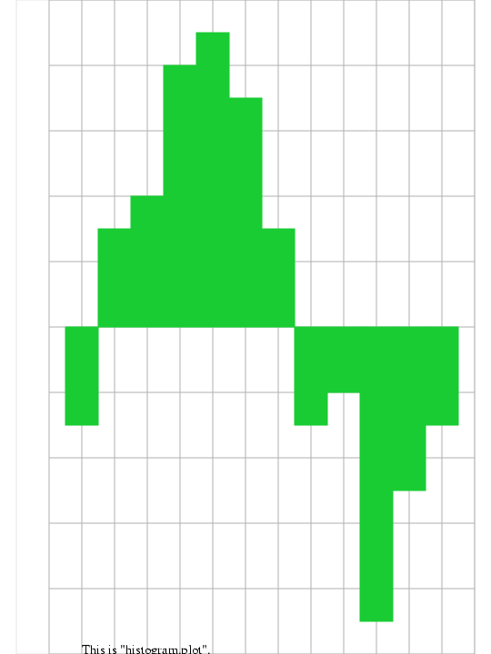
HISTOGRAM makes a histogram:

• histogram.plot, the input;
• histogram.png, the resulting PNG file.

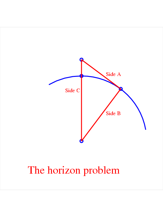
HORIZON illustrates the problem of determining the distance to the horizon:

• horizon.plot, the input;
• horizon.png, the resulting PNG file.

HULL shows some points and their convex hull:

• hull.plot, the input;
• hull.png, the resulting PNG file.

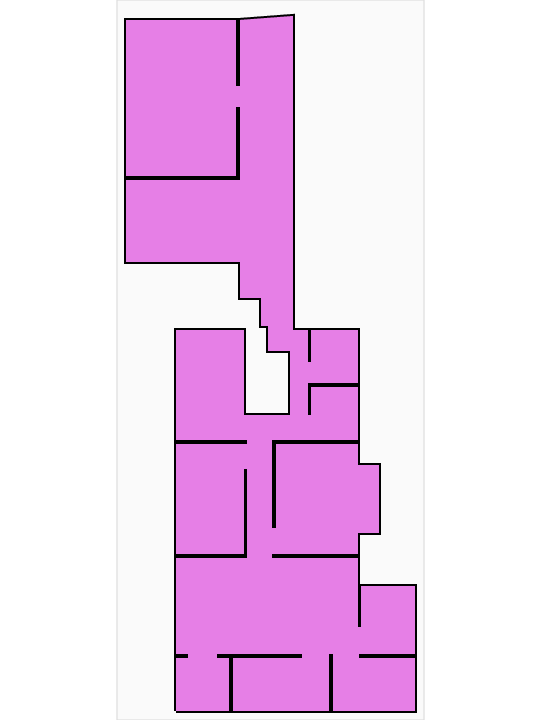
ICAM is a plan of the first floor of the Wright House.

• icam.plot, the input;
• icam.png, the resulting PNG file.

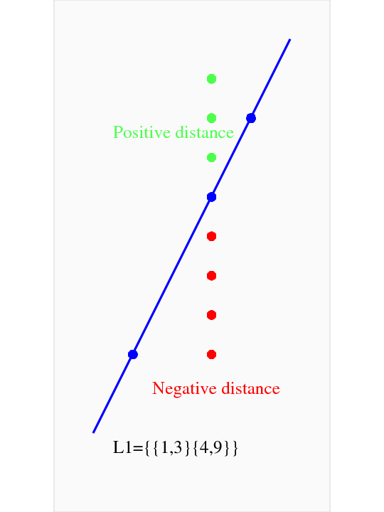
LINE_DIST shows the computation of the distance of a point from a line.

• line_dist.plot, the input;
• line_dist.png, the resulting PNG file.

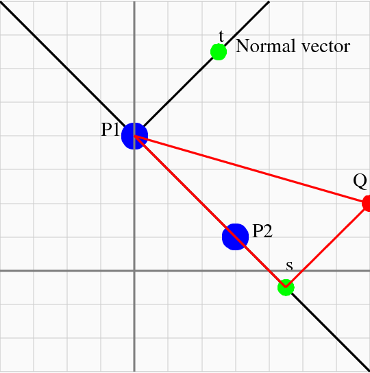
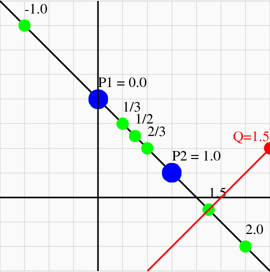
LINE_PERP shows the projection value s for points perpendicular to a line.

• line_perp.plot, the input;
• line_perp.png, the resulting PNG file.

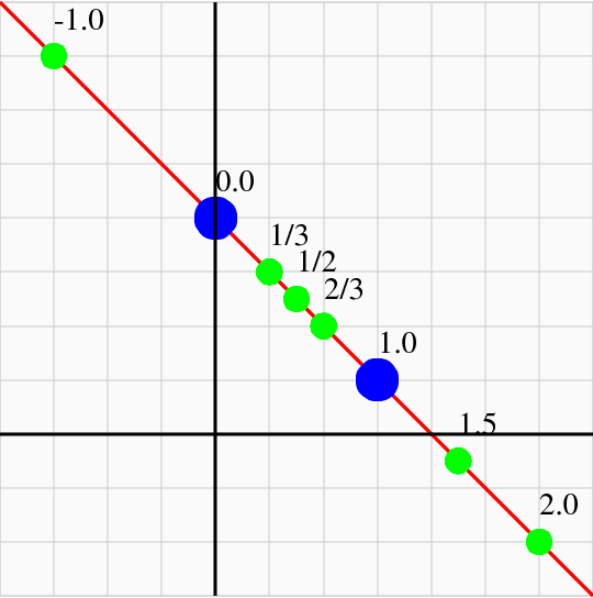
LINE_POINTS shows how the formula p=p1+s*(p2-p1) defines a line.

• line_points.plot, the input;
• line_points.png, the resulting PNG file.

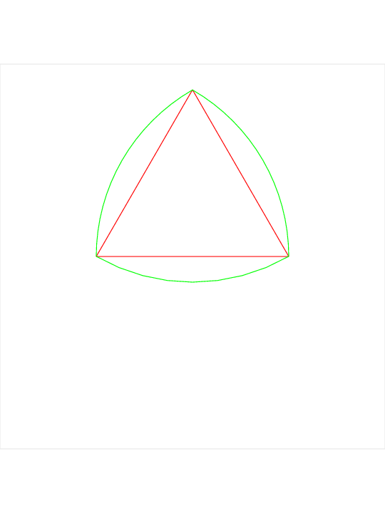
MANHOLE illustrates the construction of a curve of constant width which is not a circle:

• manhole.plot, the input;
• manhole.png, the resulting PNG file.

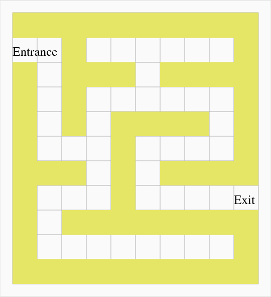
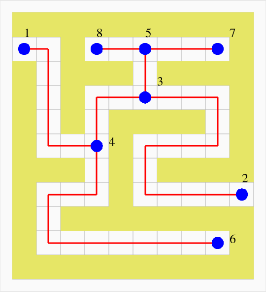
MAZE1 and MAZE2 illustrate a simple maze.

• maze1.plot, the input;
• maze1.png, the resulting PNG file.
• maze2.plot, the input;
• maze2.png, the resulting PNG file.

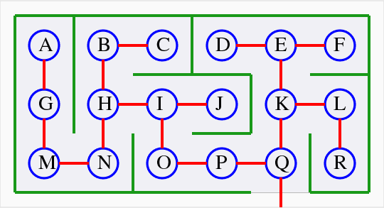
MUSEUM1 and MUSEUM2 illustrate the problem of visiting all the rooms in a museum.

• museum1.plot, the input;
• museum1.png, the resulting PNG file.
• museum2.plot, the input;
• museum2.png, the resulting PNG file.

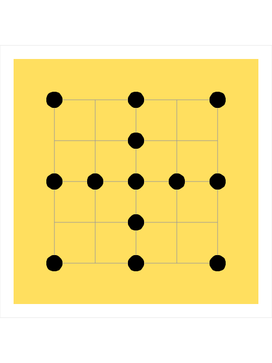
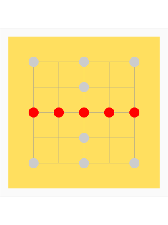
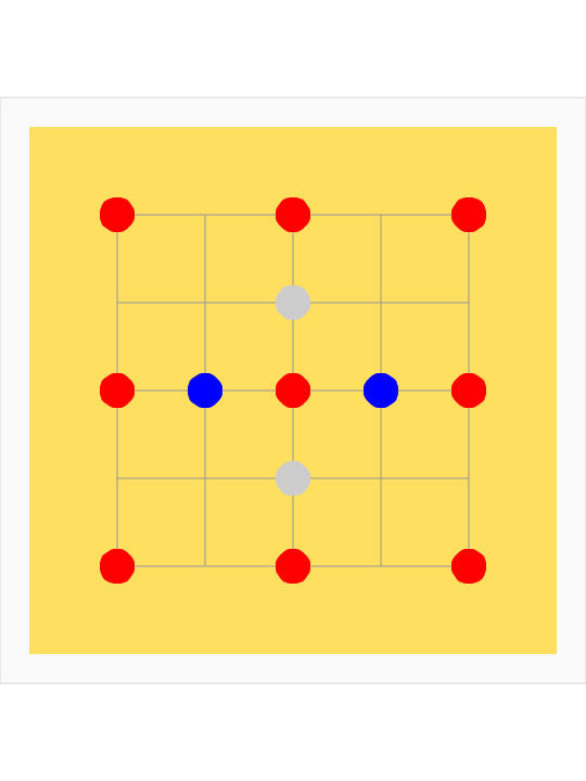
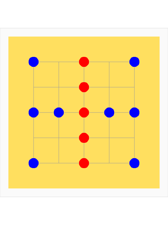
POINT_LINE_ORIENTATION illustrates the problem of the relationship of a point to a line in 2D.

• point_line_orientation.plot, the input;
• point_line_orientation.png, the resulting PNG file.

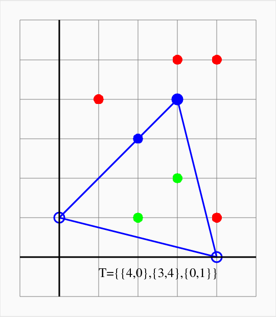
POINT_TRIANGLE_ORIENTATION illustrates the problem of the relationship of a point to a triangle in 2D.

• point_triangle_orientation.plot, the input;
• point_triangle_orientation.png, the resulting PNG file.

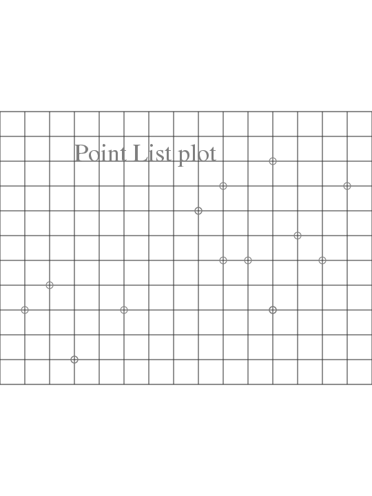
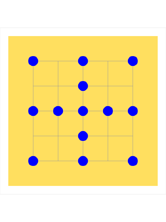
POINTS is just some points on a grid:

• points.plot, the input;
• points.png, the resulting PNG file.

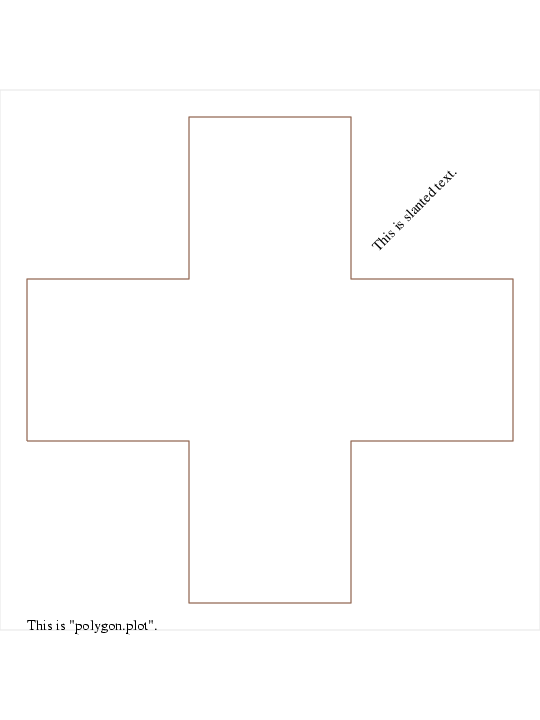
POLYGON makes a outline cross:

• polygon.plot, the input;
• polygon.png, the resulting PNG file.

POLYGON_FILL makes a gray-filled cross:

• polygon_fill.plot, the input;
• polygon_fill.png, the resulting PNG file.

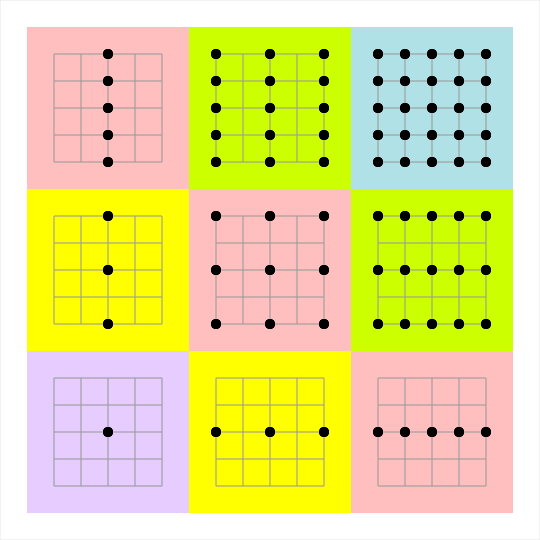
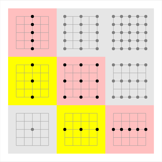
PRODUCT_GRIDS* shows a family of 2D product grids, for a talk on sparse grids.

• product_grids.plot, the input;
• product_grids.png, the resulting PNG file.
• product_grids2.plot, the input;
• product_grids2.png, the resulting PNG file.
• product_grids3.plot, the input;
• product_grids3.png, the resulting PNG file.
• product_grids4.plot, the input;
• product_grids4.png, the resulting PNG file.
• product_grids5.plot, the input;
• product_grids5.png, the resulting PNG file.
• product_grids6.plot, the input;
• product_grids6.png, the resulting PNG file.
• product_grids7.plot, the input;
• product_grids7.png, the resulting PNG file.
• product_grids8.plot, the input;
• product_grids8.png, the resulting PNG file.

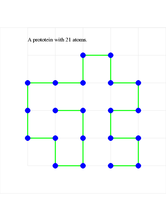
PROTOTEIN was an example of a simplified model of a protein that can fold:

• prototein.plot, the input;
• prototein.png, the resulting PNG file.

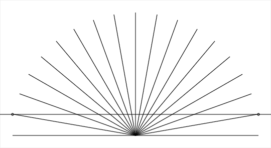
REFLECTOR is a plot used to illustrate the solution of a problem involving a "reflector". It illustrates the 'RADIUS' command:

• reflector.plot, the input;
• reflector.png, the resulting PNG file.

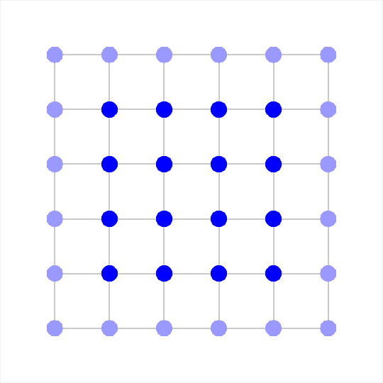
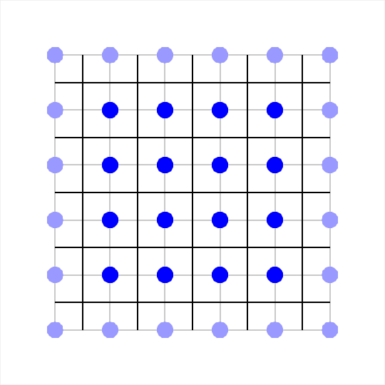
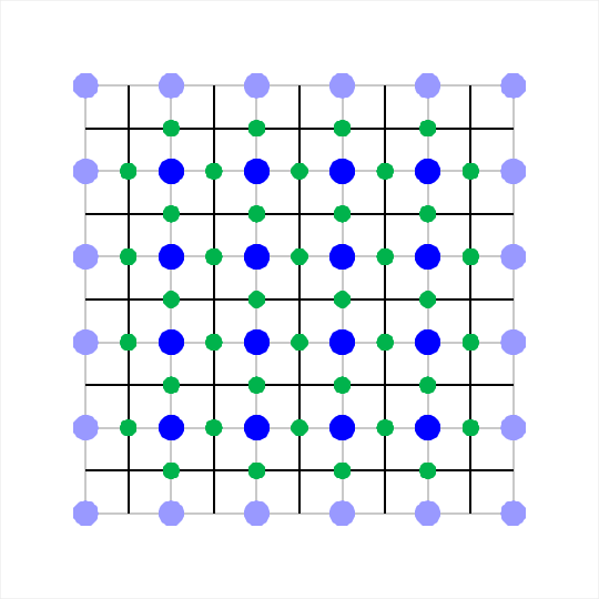
SIXBYSIX_1 a 6 by six array of dots used to illustrate a talk involving a finite difference grid.

• sixbysix_1.plot, the input;
• sixbysix_1.png, the resulting PNG file.

SIXBYSIX_2 a 6 by six array of dots used to illustrate a talk involving a finite difference grid.

• sixbysix_2.plot, the input;
• sixbysix_2.png, the resulting PNG file.

SIXBYSIX_3 a 6 by six array of dots used to illustrate a talk involving a finite difference grid.

• sixbysix_3.plot, the input;
• sixbysix_3.png, the resulting PNG file.

SIXBYSIX_4 a 6 by six array of dots used to illustrate a talk involving a finite difference grid.

• sixbysix_4.plot, the input;
• sixbysix_4.png, the resulting PNG file.

SNAKE_POLYGON illustrates a polygon to be triangulated:

• snake_polygon.plot, the input;
• snake_polygon.png, the resulting PNG file.
• snake_polygon_triangulated.plot, the input;
• snake_polygon_triangulated.png, the resulting PNG file.

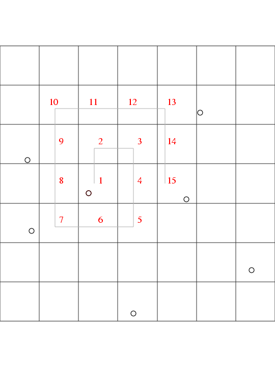
SPIRAL was an illustration of a spiral search on a grid:

• spiral.plot, the input;
• spiral.png, the resulting PNG file.

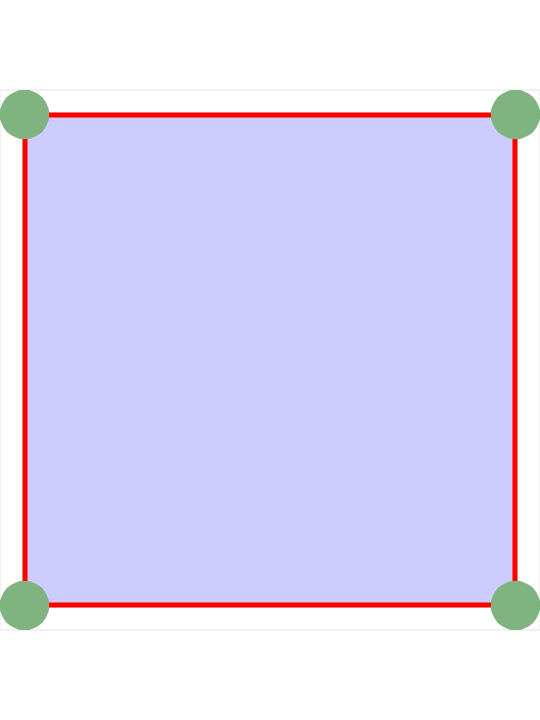
SQUARE is a square, with a blue face, thick red lines, and dark gree vertices.

• square.plot, the input;
• square.png, the resulting PNG file.

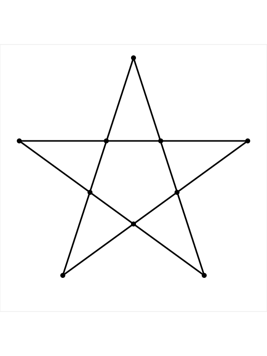
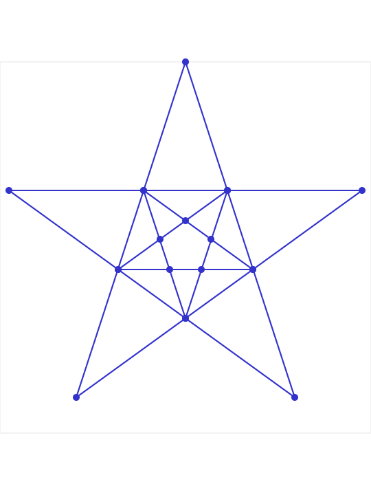
STAR is a plot of a star.

• star.plot, the input;
• star.png, the resulting PNG file.

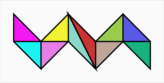
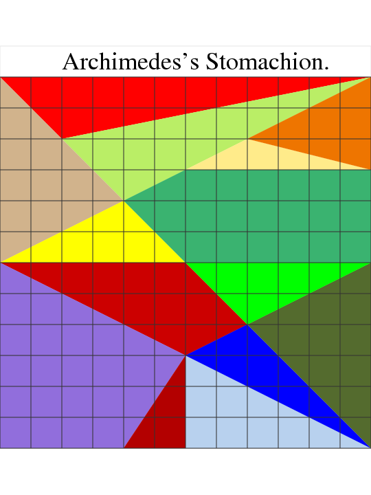
STOMACHION is a puzzle of Archimedes, involving 14 polygonal pieces that can be formed into a 12 by 12 square in 536 ways.

• stomachion.plot, the input;
• stomachion.png, the resulting PNG file.

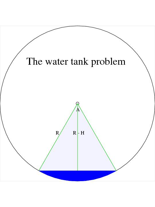
TANK is an illustration of the problem of determining the volume of a partially filled cylindrical tank:

• tank.plot, the input;
• tank.png, the resulting PNG file.

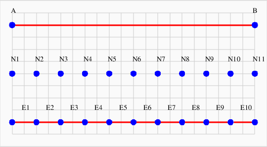
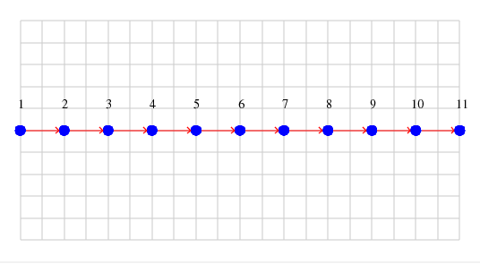
TASKS1 shows how a sequential computer carries out 11 tasks, one at a time.

• tasks1.plot, the input;
• tasks1.png, the resulting PNG file.

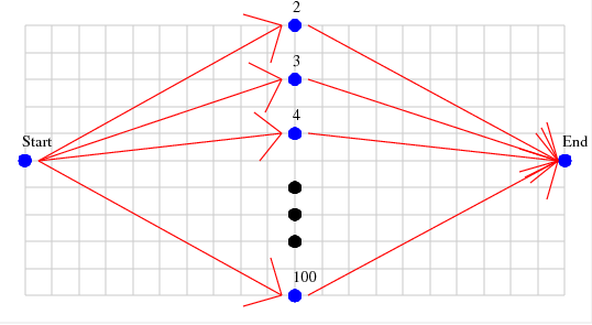
TASKS2 shows how an embarassingly parallel calculation looks.

• tasks2.plot, the input;
• tasks2.png, the resulting PNG file.

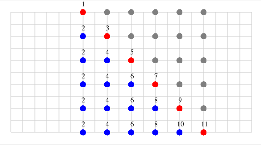
TASKS3 shows how the tasks of Gauss elimination might look to a parallel computer.

• tasks3.plot, the input;
• tasks3.png, the resulting PNG file.

TASKS4 shows how a task on a graph might look to a parallel computer.

• tasks4.plot, the input;
• tasks4.png, the resulting PNG file.
• tasks4_1.plot, the input;
• tasks4_1.png, the resulting PNG file.
• tasks4_2.plot, the input;
• tasks4_2.png, the resulting PNG file.
• tasks4_3.plot, the input;
• tasks4_3.png, the resulting PNG file.
• tasks4_4.plot, the input;
• tasks4_4.png, the resulting PNG file.
• tasks4_5.plot, the input;
• tasks4_5.png, the resulting PNG file.
• tasks4_6.plot, the input;
• tasks4_6.png, the resulting PNG file.
• tasks4_7.plot, the input;
• tasks4_7.png, the resulting PNG file.
• tasks4_8.plot, the input;
• tasks4_8.png, the resulting PNG file.

TREES1 shows how 9 trees can make lots of lines of 3:

• trees1.plot, the input;
• trees1.png, the resulting PNG file.

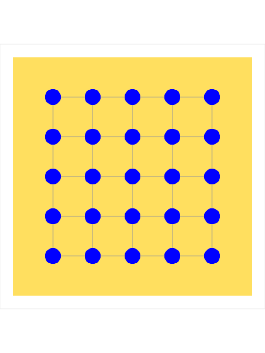
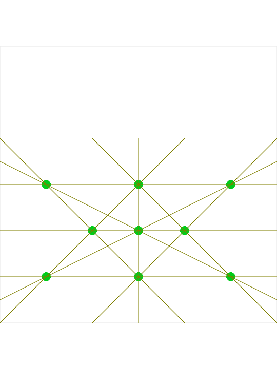
TREES2 shows how 16 trees can make lots of lines of 4:

• trees2.plot, the input;
• trees2.png, the resulting PNG file.

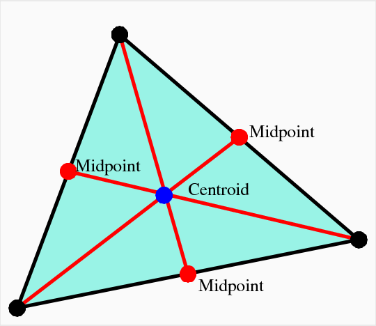
TRIANGLE_CENTROID is a plot of a triangle which suggests how the centroid is computed.

• triangle_centroid.plot, the input;
• triangle_centroid.png, the resulting PNG file.

TRIANGLE_DISTANCE illustrates the problem of determining the distance from a poiont to a (solid) triangle.

• triangle_distance.plot, the input;
• triangle_distance.png, the resulting PNG file.

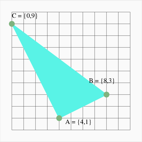
TRIANGLE_EXAMPLE1 is a plot of a triangle with the vertices labeled, used for an illustration in a discussion of triangles.

• triangle_example1.plot, the input;
• triangle_example1.png, the resulting PNG file.

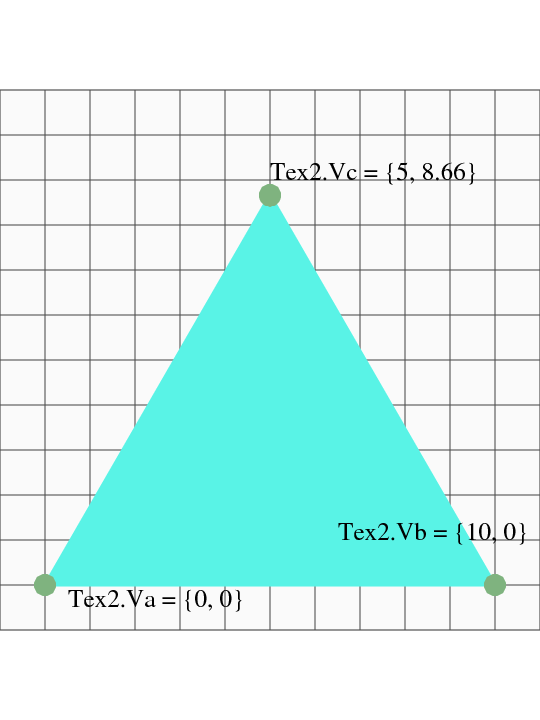
TRIANGLE_EXAMPLE2 is a plot of a triangle with the vertices labeled, used for an illustration in a discussion of triangles.

• triangle_example2.plot, the input;
• triangle_example2.png, the resulting PNG file.

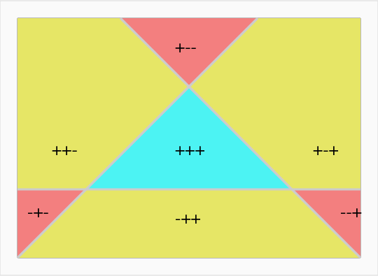
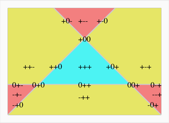
TRIANGLE_ORIENTATION shows how the sign of the three barycentric coordinates of a point determine the point's location relative to the triangle.

• triangle_orientation.plot, the input, showing only plus and minus regions.
• triangle_orientation.png, the resulting PNG file.
• triangle_orientation2.plot, the input, showing plus, zero, and minus regions;
• triangle_orientation2.png, the resulting PNG file.

TRIANGULATION_01 is a triangulation which is not maximal because a node is unused.

• triangulation_01.plot, the input;
• triangulation_01.png, the resulting PNG file.

TRIANGULATION_02 is a triangulation which is not maximal because a triangle is unused.

• triangulation_02.plot, the input;
• triangulation_02.png, the resulting PNG file.

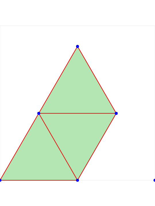
TRIANGULATION_03 is a triangulation which is maximal.

• triangulation_03.plot, the input;
• triangulation_03.png, the resulting PNG file.

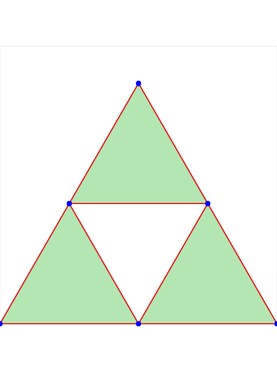
TRIANGULATION_04 is a triangulation which is not maximal because another line can be drawn, forming another triangle.

• triangulation_04.plot, the input;
• triangulation_04.png, the resulting PNG file.

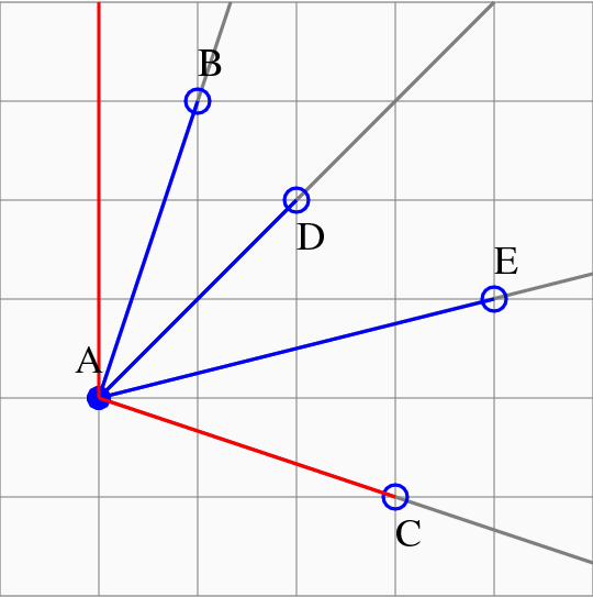
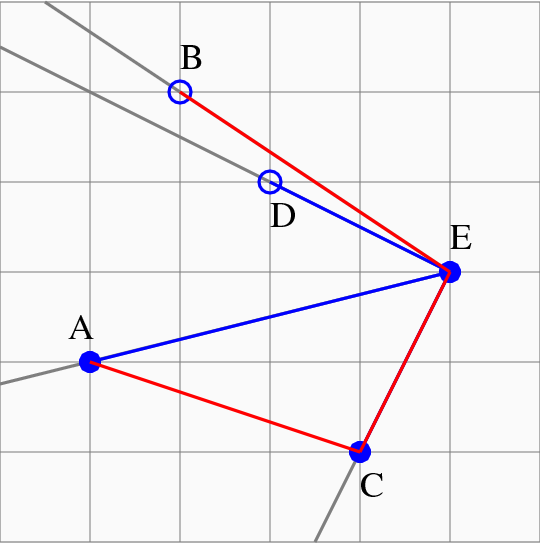
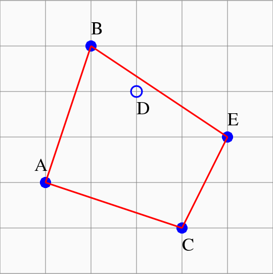
TSP_CROSSING illustrates how a portion of a proposed solution to the traveling salesman problem might exhibit a crossing.

• tsp_crossing.plot, the input;
• tsp_crossing.png, the resulting PNG file.

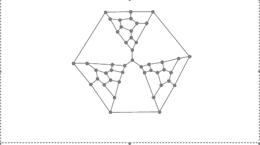
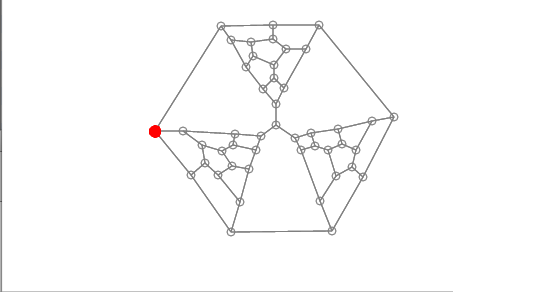
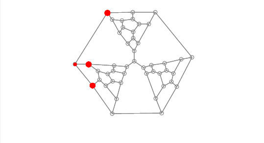
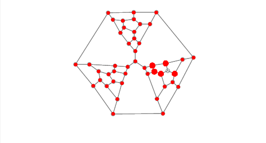
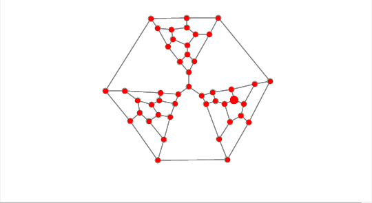
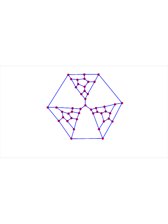
TUTTE is the Tutte graph:

• tutte.plot, the input;
• tutte.png, the resulting PNG file.

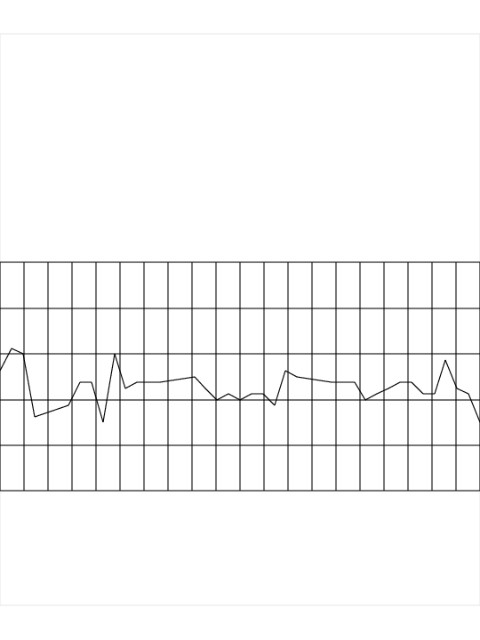
WEIGHT makes a line graph of someone's weight:

• weight.plot, the input;
• weight.png, the resulting PNG file.

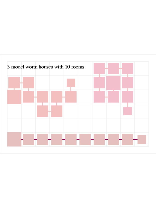
WORMS makes an illustration of some rectilinear worms on a grid:

• worms.plot, the input;
• worms.png, the resulting PNG file.

List of Routines:

• MAIN is the main program for PLOT_TO_PS.
• BOX_CLIP_LINE_2D uses a box to clip a line segment in 2D.
• CH_CAP capitalizes a single character.
• CH_EQI is a case insensitive comparison of two characters for equality.
• CH_TO_DIGIT returns the integer value of a base 10 digit.
• CIRCLE_POINTS returns N equally spaced points on a circle in 2D.
• DEGREES_TO_RADIANS converts an angle from degrees to radians.
• ELLIPSE_POINTS returns N points on an ellipse in 2D.
• FILE_NAME_EXT_GET determines the "extension" of a file name.
• FILE_NAME_EXT_SWAP replaces the current "extension" of a file name.
• GET_UNIT returns a free FORTRAN unit number.
• I4_SWAP swaps two integer values.
• POINT_INSIDE_BOX_2D determines if a point is inside a box in 2D.
• PROCESS processes the user input.
• PROCESS_HISTOGRAM processes the input defining a histogram.
• PROCESS_POLYGON processes the input defining an outlined polygon.
• PROCESS_POLYGON_FILL processes the input defining a filled polygon.
• PS_ARROW draws an arrow from (X1,Y1) to (X2,Y2).
• PS_CIRCLE draws a circle.
• PS_CIRCLE_ARC draws a circular arc.
• PS_CIRCLE_FILL draws a filled circle.
• PS_COLOR_FILL_SET sets the fill color.
• PS_COLOR_LINE handles the line color.
• PS_COLOR_LINE_SET sets the line color.
• PS_COMMENT inserts a comment into the PostScript file.
• PS_DEFAULT sets the internal settings to their default values
• PS_FILE_CLOSE closes a PostScript file.
• PS_FILE_HEAD writes header information to a PostScript file.
• PS_FILE_OPEN opens a new version of a PostScript file with a given name.
• PS_FILE_TAIL writes trailer information to a PostScript file.
• PS_FILL_GRAY sets the gray fill for polygons.
• PS_FONT_SIZE sets the font size.
• PS_GRID_CARTESIAN draws a cartesian grid.
• PS_LABEL prints a label at the current position.
• PS_LABEL_SLANT prints a slanted label at a given position.
• PS_LINE_CLOSED adds the graph of a closed line to a PostScript file.
• PS_LINE_WIDTH sets the line width.
• PS_LINETO draws a line from the current point to the given point.
• PS_MARK_CIRCLE marks a point with a small open circle.
• PS_MARK_DISK marks a point with a small filled disk.
• PS_MOVETO "moves to" a new point, which becomes the current point.
• PS_PAGE_HEAD writes header information on a new page.
• PS_PAGE_TAIL writes tail information at the end of a page.
• PS_POLYGON_FILL adds a filled polygon to a PostScript file.
• PS_SECTOR draws a circular sector.
• PS_SECTOR_FILL draws a filled circular sector.
• PS_SETTING_INT sets, gets, or prints integer internal PS_WRITE parameters.
• PS_SETTING_REAL sets, gets, or prints real internal PS_WRITE parameters.
• PS_SQUARE draws a square.
• PS_SQUARE_FILL draws a filled square.
• PS_STAR draws an open star of given radius.
• PS_STAR_CIRCLE draws open circles at the 10 points on a star of given radius.
• PS_STAR_DISK draws filled disks at the 10 points on a star of given radius.
• PS_STAR_POINTS returns 10 points on a star of given radius.
• PS_TRIANGLE draws an open triangle.
• PS_TRIANGLE_FILL draws a filled triangle.
• R8_SWAP swaps two R8's.
• S_EQI is a case insensitive comparison of two strings for equality.
• S_INDEX_LAST finds the LAST occurrence of a given substring.
• S_TO_I4 reads an I4 from a string.
• S_TO_R8 reads an R8 from a string.
• SECTOR_POINTS returns N equally spaced points on a circle in 2D.
• TIMESTAMP prints the current YMDHMS date as a time stamp.
• WORD_EXTRACT extracts the next word from a string.

You can go up one level to the FORTRAN90 source codes.