NSASM
Sparse Navier-Stokes Jacobian Assembly

NSASM is a C library which carries out the finite element assembly of the jacobian matrix used in a Newton iteration to solve the steady state incompressible Navier Stokes equations in a 2D region, by Per-Olof Persson.

The finite element approximation uses the P2-P1 triangular element, also known as the Taylor-Hood element. The velocities are approximated quadratically, and the pressures linearly.

The sparse matrix format used is known as the compressed column format, in which the nonzero entries and their row indices are stored in order by columns.

The software assumes that a suitable mesh has been set up for the region, with arrays P and T defining that mesh, that an array defining the boundary constraints has been set up, and that an initial estimate of the flow has been made available.

Invoking the Library

The software is designed to be compiled via MATLAB's mex facility. This means you have to have access to the MATLAB compiler mex; you also have to have a compiler on your computer; and you have to have (just once) set up your mex option by starting MATLAB and issuing the command "mbuild -setup".

Then you need to make a compiled copy of the nsasm code. You do this with the MATLAB command

        mex -largeArrayDims nsasm.c
      

The C code in NSASM sets up a linear system which is intended to be solved by MATLAB. Thus, the Newton iteration could have the following form in a MATLAB program:

        for ii = 1 : 8
          [ K, L ] = nsasm ( p, t, np0, e, u, mu );
          du = - lusolve ( K, L );
          u = u + du;
          disp ( sprintf ( '%20.10g  %20.10g', norm ( L, inf ), ...
            norm ( du, inf ) ) );
        end
      

Indexing Conventions

The software makes some particular assumptions about the numbering of nodes, variables, and local element nodes

(Indexing of nodes) It is assumed that the mesh was generated by starting with a set of nodes, triangulating them, and then computing the midsides of the triangles and adding these midsides to the list of nodes. In particular, the program therefore assumes that the numbering of the nodes reflects this process, so that all vertex nodes are numbered first, followed by the midside nodes.

(Indexing of global variables) It is assumed that every node has an associated horizontal velocity variable "U", that every node has an associated vertical velocity variable "V", and that only vertex nodes or "pressure nodes" have an associated pressure variable "P". The variables are stored in a single vector, first all the U's, then all the V's, then the P's. Thus variable 1 is the value of U at node 1, variable NP+1 is the value of V at node 1, and variable 2*NP+1 is the value of P at node 1.

Notice that there are even more global variables than you might think, since the boundary conditions and other constraints are handled by adding a Lagrange multiplier for each one. Thus the number of variables is actually 2*NP+NP0+NE.

(Numerical codes for U,V,P) In the E vector used to define constraints, the numeric codes 0, 1 and 2 are used for U, V and P variables respectively.

(Local numbering of nodes) When listing the 6 nodes that make up a triangle, the ordering should be as follows:

        N3
         |\
         | \
         |  \
        N5   N4
         |    \
         |     \
         |      \
        N1--N6--N2
      

Usage:

[ K, L ] = nsasm ( p, t, np0, e, u, nu );

• real P[2,NP], the coordinates of the nodes;
• integer T[6,NT], the indices of the nodes that make up the elements; the node indices are 1-based, not 0-based; the ordering of the 6 entries is vertex 1, vertex 2, vertex 3, then the node between vertex 2 and vertex 3, then the node between vertex 3 and vertex 1, and then the node between vertex 1 and vertex 2. (This is a somewhat peculiar ordering.)
• integer NP0, the number of pressure nodes, that is, nodes which are not the vertices of a triangular element.
• real E[3,NE], the constraints. Each constraint is defined by listing a node index, a variable type (0=horizonal velocity, 1 = vertical velocity, 2 = pressure), and a value to be assigned that variable.
• real U[2*NP+NP0+NE], the current estimate of the solution.
• real NU, the kinematic viscosity.
• sparse K[], a sparse matrix containing the Jacobian matrix for the Newton iteration.
• real L[2*NP+NP0+NE], the residual vector.

Languages:

NSASM is available in a C version and a FORTRAN90 version and a MATLAB version.

Related Data and Programs:

MATLAB_CALLS_C, MATLAB programs which illustrate how C functions can be written, compiled, and called from MATLAB using the mex facility;

MATLAB_CALLS_F77, MATLAB programs which illustrate how FORTRAN77 functions can be written, compiled, and called from MATLAB using MATLAB's mex facility;

MEX, MATLAB programs which call lower-level functions written in traditional languages such as C, C++, FORTRAN77 or FORTRAN90, compiled with MATLAB's mex compiler.

MSM_TO_HB, a MATLAB program which writes a MATLAB sparse matrix to a Harwell Boeing (HB) file, by Xiaoye Li.

SUPERLU, a C library which applies a fast direct solution method to a sparse linear system, by James Demmel, John Gilbert, and Xiaoye Li.

Author:

Original C+MATLAB version by Per-Olof Persson.
This C+MATLAB version by John Burkardt.

Reference:

1. Klaus-Juergen Bathe,
   Finite Element Procedures,
   Prentice Hall, 1996.
2. James Demmel, John Gilbert, Xiaoye Li,
   SuperLU User's Guide,
   September, 1999.
3. Per-Olof Persson,
   Implementation of Finite Element-Based Navier-Stokes Solver,
   April 2002.
4. Michael Schaefer, Stefan Turek,
   Benchmark Computations of Laminar Flow Around a Cylinder,
   Notes on Numerical Fluid Mechanics,
   Volume 52, 1996, pages 547-566.

Source Code:

The C source code carries out the assembly of the finite element matrix and residual. To use it, you must compile it once. To do that, you need to set up mex (once), run matlab, and issue the command

        mex -largeArrayDims nsasm.c
      

Since the file is C code, you could instead compile it with any standard C compiler, but you will need to access the MEX include files invoked in the file. The location of these include files depends on how your copy of MATLAB was installed.

• nsasm.c, the source code.

The MATLAB source code comprises just a couple of utility routines to be called by the MATLAB test programs.

• nsasm_interface.m, reads node, element and constraint data from files whose names are specified by the user, and calls the nsasm function to compute the stiffness matrix K and residual L.
• r8sp_print_some.m, prints part of a sparse triplet matrix.
• timestamp.m, prints the current YMDHMS date as a timestamp.

Examples and Tests:

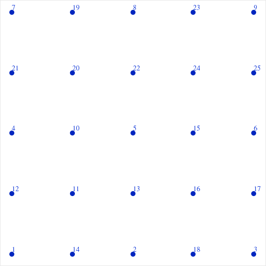
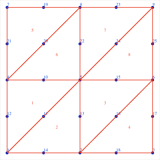
The SMALL test defines a small sparse matrix, with NP = 25 nodes, NT = 8 elements, NE = 33 constraints, NP0 = 9, NU = 100.0.

• nsasm_test_small.m, calls nsasm_interface() for the "small" data.
• nsasm_test_small_output.txt, the printed output.
• small_constants.txt, records the constants for the problem, NP, NT, NE, NP0, NU.
• small_constraints.txt, the constraint file (3*33 entries), sets to zero the horizontal and vertical velocities at the 16 boundary nodes, and sets 1 pressure to 0.
• small_nodes.txt, the point coordinate file, 25 nodes.
• small_nodes.png, a PNG image of the nodes.
• small_elements.txt, the element file, 8 quadratic (6 node) triangles.
• small_elements.png, a PNG image of the elements.
• small.hb, a Harwell-Boeing file containing a copy of the matrix and right hand side in a compressed format.

The BIG_CONSTRAINT_FILE_MAKER program was set up because I lost or never had a copy of the "big_constraints.txt" file, and I had to guess the problem type (driven cavity) and the location of the boundary nodes on left, bottom and right, and then manufacture the appropriate constraint data:

• big_constraint_file_maker.m, reads "big_nodes.txt" and creates "big_constraints.txt".
• big_constraint_file_maker_output.txt, the printed output.

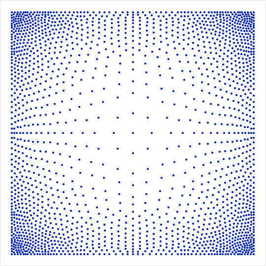
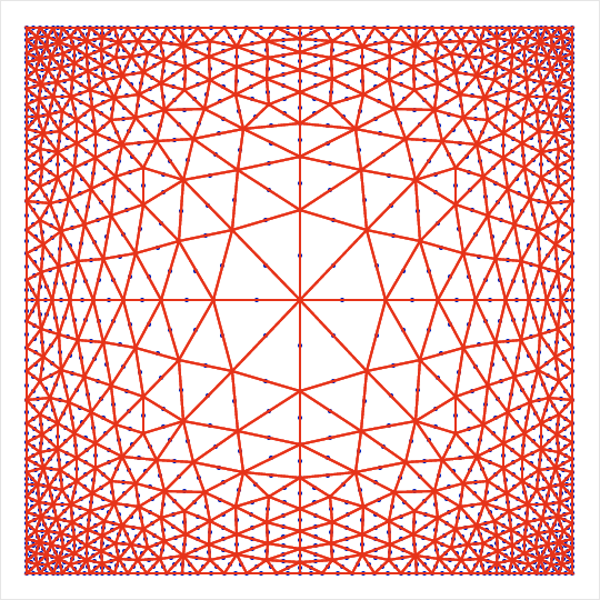
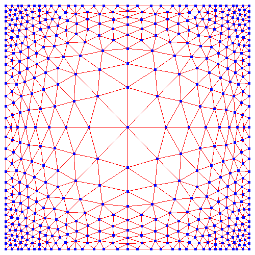
The BIG test defines a relatively large sparse matrix, with NP = 2049 nodes, NT = 960 elements, NE = 387 constraints, NP0 = 545, NU = 500.0, a version of the driven cavity problem, with an unstructured mesh.

• nsasm_test_big.m, calls nsasm_interface() for the "big" data.
• nsasm_test_big_output.txt, the printed output.
• big_constants.txt, records the constants for the problem, NP, NT, NE, NP0, NU.
• big_constraints.txt, the constraint file (3*1287 entries).
• big_nodes.txt, the point coordinate file, 2049 nodes.
• big_nodes.png, a PNG image of the nodes.
• big_elements.txt, the element file, 960 quadratic (6 node) triangles.
• big_elements.png, a PNG image of the elements.
• big.hb, a Harwell-Boeing file containing a copy of the matrix and right hand side in a compressed format.

The element data for the big problem is quadratic, and the assumption is made that the midside nodes are the midpoints of the corresponding vertices. That is, the 6-noded triangles have straight sides, with the mid-side nodes actually at the geometric middles of their sides. The easiest way to guarantee such a triangulation is to generate a triangulation with 3-noded triangles, and then generate the midside nodes in the obvious way. Here we include the original 3-noded triangulation information.

• big_linear_nodes.txt, the nodes for the linear triangulation.
• big_linear_elements.txt, the elements for the linear triangulation.
• big_linear_elements.png, the elements for the linear triangulation.

List of Routines:

The C file nsasm.c contains the following functions:

• mexFunction is the interface between MATLAB and the C code.
• ASSEMBLE assembles the local stiffness and residual into global arrays.
• ASSEMBLE_CONSTR assembles the constraints.
• INIT_SHAPE evaluates the shape functions at the quadrature points.
• IVEC_HEAP_D reorders an array of integers into a descending heap.
• IVEC_SORT_HEAP_A ascending sorts an array of integers using heap sort.
• LOCALKL assembles the local stiffness matrix and residual.
• SPARSE_CREATE creates a sparse matrix.
• SPARSE_SET increments an entry of the sparse matrix.

You can go up one level to the C source codes.