Definition (Intuitive Definition of Limits)

When we say that  we mean that for all values of  near (but different from) , then the function values  are all near .

>

Outline

• Graphical Evaluation of Limits
• Basic Analytic Methods
• Piecewise-Defined Functions and One-Sided Limits
• Two Special Trigonometric Limits
• Graphs and Tables can be Misleading
• Limits for Oscillating Functions

>

Example 1:  

>	f1 := ( x^4 - 13*x^3 + 62*x^2 - 120*x + 64 ) / ( x - 4 ): f(x) = f1;

Prior to evaluating any limits, it is adviseable to plot the function. In this case, notice that the function is not defined for x=4.

>

p1 := display( [plot( f1, x=0..3.95 ),                 plot( f1, x=4.05..6 ),                 pointplot( [4,8], symbol=circle, symbolsize=18),                 pointplot( [1,2], symbol=cross, symbolsize=18, color=blue)] ): display( p1, title="Example 1: Plot of y=( x^4 - 13*x^3 + 62*x^2 - 120*x + 64 ) / ( x - 4 ) on [0,6]" );

>

The first attempt when evaluating a limit is to attempt to evaluate the function at the limit point. In this case, the function is defined at  (see the blue cross in the above plot), and the value of the function at  is

>	eval( f1, x=1 );

Based on this computation, and the graph, it appears as though

>	Limit( f1, x=1 ) = eval( f1, x=1 );

To confirm this result, note that Maple reports the value of this limit to be

>	Limit( f1, x=1 ) = limit( f1, x=1 );

>

The same technique could be applied to all other limit points --- except . At  this function is not defined. From the graph it is clear that all function values close to  approach the same value, namely 5. An analytic derivation for this result will be developed next.

Example 2:  

>	f1 := ( x^4 - 13*x^3 + 62*x^2 - 120*x + 64 ) / ( x - 4 ): f(x) = f1; p1 := display( [ plot( f1, x=0..3.95 ),                  plot( f1, x=4.05..6 ),                  pointplot( [4,8], symbol=circle, symbolsize=18) ] ):

The first attempt when evaluating a limit is to evaluate the function at the limit point. In this case, the function is not defined at :

>	eval( f1, x=4 );

Error, numeric exception: division by zero

Upon closer inspection it is seen that both numerator and denominator are zero when :

>	eval( numer(f1), x=4 ); eval( denom(f1), x=4 );

This means that we can factor ( ) from both numerator and denominator. The resulting function is

>	n1 := factor( numer(f1) ); d1 := factor( denom(f1) ); f2 := n1/d1;

The new function, f2 , is identical to f1  except that it is defined at . This can be illustrated in a plot.

>	p2 := plot( f2, x=0..6, color=green, thickness=3 ): display( [p1,p2], title="Example 2: Plot of\ny=(x^4-13*x^3+62*x^2-120*x+64)/(x-4) and y=x^3-9*x^2+26*x-16\non [0,6]" );

The goal of this example is to illustrate that changing the definition of the function at one point does not change the value of the limit:

>	Limit( f1, x=4 ) = Limit( f2, x=4 );

The limit can be evaluated as in the previous example:

>	Limit( f2, x=4 ) = eval( f2, x=4 );

This result appears to be consistent with the graphical information. Moreover, Maple reports the value of the original limit to be

>	Limit( f1, x=4 ) = limit( f1, x=4 );

Example 3:  

>	f3 := piecewise( x<1, -x^2+2, x>=1, sqrt(x-1)-2*x/3+2 ): f(x) = f3;

As before, we begin with a plot

>	p3 := plot( f3, x=0..6, discont=true ): display( p3, view=[0..6,0..3], title="Example 3: Plot of a piecewise-defined function with a jump at x=1" );

This picture convincingly shows that the (two-sided) limit of this function does not exist at . This is true even though there is no problem directly evaluating the function at the limit point:

>	eval( f3, x=1 );

but Maple reports that the limit does not exist

>	limit( f3, x=1 );

To understand why this limit does not exist, consider the two one-sided limits:

>	q1 := Limit( f3, x=1, left ) = Limit( -x^2+2, x=1 ): q1,`` = eval( -x^2+2, x=1 );

>	q2 := Limit( f3, x=1, right ) = Limit( sqrt(x-1)-2*x/3+2, x=1 ): q2; `` = eval( sqrt(x-1)-2*x/3+2, x=1 );

The fact that the one-sided limits have different values explains why the two-sided limit does not exist. This result is confirmed by Maple:

>	q3 := Limit( f3, x=1 ): q3 = value( q3 );

>

Example 4:  

>	f4 := piecewise( x<1, -x^2+2, x>=1, sqrt(x-1)-x+2 ): f(x) = f4;

This function looks very similar to the function in Example 3. A plot shows that there is, however, a fundamental difference:

>	p4 := plot( f4, x=0..6, discont=true ): display( p4, view=[0..6,0..3], title="Example 4: Plot of piecewise-defined function without a jump" );

This picture suggests that the values of this function on either side of  approach the same value -- namely, 1. To confirm this, look at the two one-sided limits:

>	q1 := Limit( f4, x=1, left ) = Limit( -x^2+2, x=1 ): q1; `` = eval( -x^2+2, x=1 );

>	q2 := Limit( f4, x=1, right ) = Limit( sqrt(x-1)-x+2, x=1 ): q2; `` = eval( sqrt(x-1)-x+2, x=1 );

The fact that the one-sided limits exist and have the same value permits us to conclude the two-sided limit does exist and has value 1. Maple confirms this conclusion:

>	q3 := Limit( f4, x=1 ): q3 = value( q3 );

>

Example 5:  

>	f5 := sin(3*x)/(4*x): f(x) = f5;

Observe that this function is not defined for  and no amount of factoring or other manipulation can eliminate the "division by zero" problem at . In situations like this the graph is even more important.

>	p5 := display( [ plot( f5, x=-Pi..-0.05 ),                  plot( f5, x=0.05..Pi ),                  pointplot( [0,0.75], symbol=circle, symbolsize=18) ] ): display( p5, view=[-Pi..Pi,-0.25..1], title="Plot of y=sin(3*x)/(4*x) on [-Pi,Pi]" );

This plot suggests that the limit should exist and its value should be around 0.75. To gather further evidence in support of this observation, create a table of values for the function evaluated close to zero.

>	a := 0: H := [ 1.0, 0.5, 0.1, 0.01, 0.001, 0.0001, 0.00001 ]:

For values converging to  from the left of the limit point:

>	xL := [seq( a-h, h=H )]: bodyL := seq( < X | eval(f5,x=X) >, X=xL ): header := < theta | f(theta) >, <`_______` | `____________` >: < header, bodyL >;

>

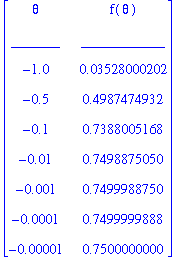
This suggests that the one-sided limit from the left exists and has value .

>

Similarly, for values converging to  from the right of the limit point:

>	xR := [seq( a+h, h=H )]: bodyR := seq( < X | eval(f5,x=X) >, X=xR ): < header, bodyR >;

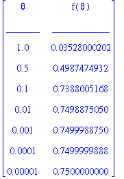
supports the claim that the one-sided limit from the right exists and has value .

>

The existence and agreement of both one-sided limits is additional support for the claim that the value of the (two-sided) limit is 3/4.

>

Example 6:  

>	f6 := (100*x - cos(x))^2/100000: f(x) = f6;

>

As usual, begin with a plot of the function. The graph of  is included for comparison purposes.

>	p6 := plot( [f6,x^2/10-x/500], x=-1..1, thickness=[1,3] ): display( p6, title="Plot of y=(100*x-cos(x))^2/100000 and y=x^2/10-x/500 on [-1..1]" );

The graph of this function is indistinguishable from the graph of  on this interval.

>

If we create tables of function values for this function to the left and right of , we might obtain

>	a := 0: H := [ 1.0, 0.5, 0.1, 0.01 ]: xL := [seq( a-h, h=H )]: xR := [seq( a+h, h=H )]:

For values converging to  from the left of the limit point:

>	header := < `x` | `f(x)` >, < `_____` | `_______________` >: bodyL := seq( < X | eval( f6, x=X ) >, X= a-H ): tableL := < header, bodyL >:

and from the right of the limit point:

>	bodyR := seq( < X | eval( f6, x=X ) >, X= a+H ): tableR := < header, bodyR >: tableL, tableR;

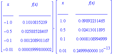
The most likely conjecture about this limit based on these (short) lists of function values is that . However, this is incorrect.

This limit can be evaluated by direct evaluation of this function at . This operation yields

>	q1 := Limit( f6, x=0 ) = eval( f6, x=0 ): q1; `` = evalf( eval(f6,x=0) );

which is in agreement with Maple

>	q2 := Limit( f6, x=0 ): q2 = value( q2 );

>

Thus, the initial picture and subsequent tables were all misleading. In this case if we zoom in on the graph to the interval [-0.01, 0.01 ], the functions are seen to be quite different.

>	p6z := plot( [f6,x^2/10-x/500], x=-0.01..+0.03, thickness=[1,3] ): display( p6z, title="Plot of y=(100*x-cos(x))^2/100000 and y=x^2/10-x/500 on [-0.01..0.03]" );

The point of this example is to illustrate that neither a graph nor a table of function values can completely justify the evaluation of a limit. Graphs of the function and corresponding tables of values can be useful but are only the first step. Hopefully, the information gathered from the table of function values suggests other methods and techniques for justifying the evaluation of a limit. The rigorous evaluation of limits is discussed in the Precise Definition of the Limit lesson.

>

Example 7:  

>	f7 := sin(1/x): f(x) = f7;

This function is not defined at . A graph of the function that avoids the problems at the origin shows that this function oscillates between -1 and 1.

>	p7 := display( [ plot( f7, x=-2/Pi..-0.01 ),                  plot( f7, x= 0.01.. 2/Pi ) ] ): display( p7, title="Plot of y=sin(1/x) on [-2/Pi,2/Pi]" );

>

Observe that the period of the oscillations increases as the points move closer to the origin -- from both the left and the right. This suggests that the function will take on all values between -1 and 1 infinitely often for points close to . In particular, the value of the function does not approach a single point and the limit (two-sided or one-sided) does not exist.

>

Observe that Maple's evaluation of this limit informs us that the limit does not exist and the reason for this is that the values oscillates between -1 and 1.

>	q1 := Limit( f7, x=0 ): q1 = value( q1 );

>

A Concept-Based Approach to Evaluating