lab7.mws --- Limits, l'Hopital's Rule, and Rates of Growth, "e" gads!
| > |
restart;
with( plots ):
|
Warning, the name changecoords has been redefined
Lab Overview
Why are we taking time to develop l'Hopital's rule? Part of the answer is that the method does not make sense until you know about derivatives. Another part of the reason is that the indeterminate forms that can be evaluated with l'Hopital's rule are going to appear in several contexts within the next month or so of this course. The limits encoutnered in this lab have been selected specifically for their importance later in this course.
Maple's
limit
command can evaluate almost any limit we are likely to ever encounter. l'Hopital's rule is applied automatically whenever it is needed. Simply using this command does not help us develop our understanding of limits. The
Limit
maplet [
Maplet Viewer][
MapleNet] is a Java-based graphical interface written in Maple that allows us to focus on selecting appropriate techniques to evaluate integrals. While this maplet is similar to the Integration maplet [
Maplet Viewer][
MapleNet], it is not nearly as useful and will not be utilized explicitly in this lab. It is mentioned here for your information. Check it out if you are interested.
Except for the essay question, the questions for this lab are either taken from the assigned homework problems or other problems in the textbook.
Deadline for submitting a lab solution is midnight, Thursday, February 27, 2003.
Example 1:
 (p. 407, # 4)
Let's start with a problem that is not at all obvious.
| > |
F := arctan(3*x)/arcsin(x):
L := Limit( F, x=0 ):
L;
|

When you first look at this problem, and note that
 , it is difficult to know where to start. Most people just do not have the familiarity with the inverse trigonometric functions to be able to "see" the value of this limit. To begin to understand the problem, plot the function
 on an interval containing the origin. Because the arcsin function is defined only on
![`union`(`[-1,0)`,`(0,1]`)](images/lab75.gif) , that is the largest domain on which this function is defined.
, that is the largest domain on which this function is defined.
| > |
p1 := plot( F, x=-1..-0.01, y=0..5 ):
p2 := plot( F, x=0.01..1, y=0..5 ):
display( [p1,p2] );
|
![[Maple Plot]](images/lab76.gif)
The plot suggests that the value of the limit will be 3. Let's see if we can confirm this using properties of limits. Because the denominator converges to 0 as x->0 there is a hope that l'Hopital's rule will apply. To check this, obtain the numerator and denominator and check their limits as
 ->0:
->0:
| > |
f := numer(F):
Lf := Limit( f, x=0 ):
Lf = value( Lf );
|

| > |
g := denom(F):
Lg := Limit( g, x=0 ):
Lg = value( Lg );
|

Because this limit has form
 , l'Hopital's rule can be applied. The derivatives of the numerator and denominator are
| > |
f1 := Diff( f, x ):
g1 := Diff( g, x ):
f1 = value( f1 );
g1 = value( g1 );
|


so
| > |
F1 := value( f1/g1 ):
f1/g1 = F1;
|

The original limit can be replaced by
| > |
L1 := Limit( F1, x=0 ):
L1;
|

This limit is easy to evaluate:

Thus, as predicted from the plot,
| > |
L = L1;
`` = eval( F1, x=0 );
|


To conclude, let's look at the plot of the two functions considered in this problem.
| > |
p3 := plot( F1, x=-1..1, y=0..5, color=green ):
display( [p1,p2,p3] );
|
![[Maple Plot]](images/lab718.gif)
Note that the functions are different, but do have the same limit at
 .
.
Example 2:

The function
| > |
F := x*ln(x):
`F(x)`=F;
|

is defined only for
 > 0. A plot of this function on an interval to the right of the origin
| > |
p1 := plot( F, x=0.01..3 ):
p1;
|
![[Maple Plot]](images/lab723.gif)
suggests that
| > |
L := Limit( F, x=0, right ):
L = 0;
|

Now, let's see if we can confirm this. The original limit is has indeterminate form
 . To apply l'Hopital's rule it is necessary to convert this to a
 or
or
 form. This can be done by writing the original problem as either
 =
=
 (
(
 )
)
or
 =
=
 (
(
 )
)
The first form looks more appealing because it is easier to differentiate
 than
than
 . To verify that l'Hopital's rule applies
| > |
f := ln(x):
Lf := Limit( f, x=0, right ):
Lf = value( Lf );
|

| > |
g := 1/x:
Lg := Limit( g, x=0, right ):
Lg = value( Lg );
|

Applying l'Hopital's rule means computing derivatives
| > |
f1 := Diff( f, x ):
g1 := Diff( g, x ):
f1 = value( f1 );
g1 = value( g1 );
|


so
| > |
F1 := value( f1/g1 ):
f1/g1 = F1;
|

The original limit can be replaced by
| > |
L1 := Limit( F1, x=0, right ):
L1;
|

This limit is easy to evaluate:

Thus, as predicted from the plot,
| > |
L = L1;
`` = eval( F1, x=0 );
|


To conclude, let's look at the plot of both functions considered in this problem.
| > |
p2 := plot( F1, x=0..1, color=green ):
display( [p1,p2] );
|
![[Maple Plot]](images/lab745.gif)
Note that the functions are different, but do have the same limit at
 .
.
Example 3:
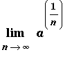 (
(
 > 0)
> 0)
The limit variable,
 , is assumed to be an integer. In this form, l'Hopital's rule is not applicable. The usual approach to this problem is to convert the problem to an equivalent problem involving a real variable. In most situations this is done by simply replacing all occurrences of
 with
with
 :
:
| > |
Ln := Limit( a^(1/n), n=infinity ):
Lx := Limit( a^(1/x), x=infinity ):
Ln = Lx;
|

To emphasize that these problems are equivalent -- and to gain insight into the value of this limit -- consider the following plot. This plot contains the
| > |
G := (a,n) -> a^(1/n):
p1 := plot( [seq([n,G(5,n)],n=1..10 )], style=point, color=blue,
view=[0..10,0..5], legend=["a=5, discrete points"] ):
p2 := plot( G(5,x), x=1..10, color=cyan,
legend=["a=5, continuous variable"] ):
p3 := plot( [seq([n,G(1/5,n)],n=1..10 )], style=point, color=red,
view=[0..10,0..5], legend=["a=1/5, discrete points"] ):
p4 := plot( G(1/5,x), x=1..10, color=pink,
legend=["a=1/5, continuous variable"] ):
display([p1,p2,p3,p4]);
|
![[Maple Plot]](images/lab753.gif)
Evaluation of this integral, for any
 > 0, begins by rewriting
 =
=
 =
=

Then,
 =
=
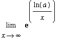 =
=
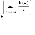 .
.
The limit that interests us now is
| > |
L := Limit( ln(a)/x, x=infinity ):
L;
|

In this limit, the denominator has a limit of
 while the numerator has a finite limit that can be either positive (
 > 1), negative (0 <
 < 1 ) or zero (
 = 1 ). This is not an indeterminate form;
l'Hopital's rule cannot be applied!
However, it is easily seen that
 =
=
 =
=
 = 0
= 0
To conclude,
 =
=
 =
=
 = 1.
= 1.
This is consistent with the plot.
Example 4:
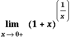
This problem has an indeterminate form of
 . L'Hopital's rule can be used only after it has been rewritten with an indeterminate form of
 or
or
 . Prior to rewriting the problem, however, let's see if a plot can suggest if this limit exists and what its value might be.
| > |
plot( (1+x)^(1/x), x=0.01..10, y=0..3 );
|
![[Maple Plot]](images/lab776.gif)
This picure suggests the limit exists and has a value around 2.7.
To rewrite this problem in a form suitable for l'Hopital's rule, note
 =
=
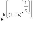 =
=
 .
.
This means
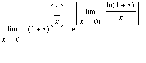
In the new limit
| > |
F := ln(1+x)/x:
L := Limit( F, x=0, right ):
L;
|

the fact that the numerator and denominator satisfy
| > |
f := numer( F ):
Lf := Limit( f, x=0, right ):
Lf = value( Lf );
|

| > |
g := denom( F ):
Lg := Limit( g, x=0, right ):
Lg = value( Lg );
|

means this limit has indeterminate form 0/0. An application of l'Hopital's rule leads to
| > |
f1 := Diff( f, x ):
g1 := Diff( g, x ):
f1 = value( f1 );
g1 = value( g1 );
|


so
| > |
F1 := value( f1/g1 ):
f1/g1 = F1;
|

The original limit can be replaced by
| > |
L1 := Limit( F1, x=0, right ):
L1;
|

This limit is easy to evaluate:

Thus,
| > |
L = L1;
`` = eval( F1, x=0 );
|


and so, the original limit is
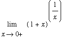 =
=
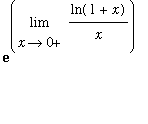 =
=
 =
=

To conclude, note that
| > |
exp(1) = evalf(exp(1));
|

which is consistent with the conjecture made at the beginning of this problem.
Example 5:
Note: Essay Question
This example should help you to answer the Essay Question.
As
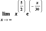
 increases without bound, the power function increases rapidly and the exponential decays to zero. What happens to their product? This problem begs for a plot, but how do we look at the behavior at infinity?
| > |
F := x^(5/2) * exp(-x/30):
P1 := plot( F, x=0..10 ):
P1;
|
![[Maple Plot]](images/lab798.gif)
Based on this picture, it looks like the function might increase forever. But, 10 is not a very big number.
| > |
P2 := plot( F, x=0..100 ):
P2;
|
![[Maple Plot]](images/lab799.gif)
Now it is clear that something more happens but we are not yet in a position to say anything about the limit at
 .
.
| > |
P3 := plot( F, x=0..1000 ):
P3;
|
![[Maple Plot]](images/lab7101.gif)
This is a little more convincing - but how do we know nothing different happens for
 > 1000?
Initial Analysis
The limit has indeterminate form
 . This can be converted to the form
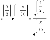
 by writing
 .
.
| > |
f := x^(5/2):
Lf := Limit( f, x=infinity ):
Lf = value( Lf );
|

| > |
g := exp(x/30):
Lg := Limit( g, x=infinity ):
Lg = value( Lg );
|

First Application of l'Hopital's Rule
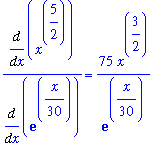
Applying l'Hopital's rule means computing the derivatives
| > |
f1 := Diff( f, x ):
g1 := Diff( g, x ):
f1 = value( f1 );
g1 = value( g1 );
|


so
| > |
F1 := value( f1/g1 ):
f1/g1 = F1;
|
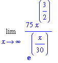
The original limit can be replaced by
| > |
L1 := Limit( F1, x=infinity ):
L1;
p1 := plot( F1, x=0..1000, color=green ):
display( [P3, p1] );
|
![[Maple Plot]](images/lab7112.gif)
This limit is not easily evaluated. In fact, it has indeterminate form
 :
:
| > |
Lf1 := Limit( f1, x=infinity ):
Lf1 = value( Lf1 );
|

| > |
Lg1 := Limit( g1, x=infinity ):
Lg1 = value( Lg1 );
|

Second Application of l'Hopital's Rule
A second application of l'Hopital's rule means computing the second derivatives
| > |
f2 := Diff( f1, x ):
g2 := Diff( g1, x ):
f2 = value( f2 );
g2 = value( g2 );
|


so
| > |
F2 := value( f2/g2 ):
f2/g2 = F2;
|
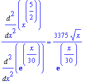
The new limit to be considered is
| > |
L2 := Limit( F2, x=infinity ):
L2;
p2 := plot( F2, x=0..1000, color=blue ):
display( [P3,p1,p2] );
|

![[Maple Plot]](images/lab7120.gif)
This limit is somewhat simpler, but still is indeterminate with form
 .
.
| > |
Lf2 := Limit( f2, x=infinity ):
Lf2 = value( Lf2 );
|

| > |
Lg2 := Limit( g2, x=infinity ):
Lg2 = value( Lg2 );
|

Third Application of l'Hopital's Rule
A third application of l'Hopital's rule means computing the third derivatives
| > |
f3 := Diff( f2, x ):
g3 := Diff( g2, x ):
f3 = value( f3 );
g3 = value( g3 );
|


so
| > |
F3 := value( f3/g3 ):
f3/g3 = F3;
|
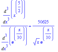
Aha! Now we are getting somewhere! This limit is not an indeterminate form. In fact, the numerator is finite and the denominator increases without bound (as x increases towards infinity).
The original limit can be replaced by
| > |
L3 := Limit( F3, x=infinity ):
L3;
p3 := plot( F3, x=0..1000, color=cyan ):
display( [P3,p1,p2,p3] );
|

![[Maple Plot]](images/lab7128.gif)
Each limit encountered in the application of l'Hopital's rule appears to have a limit of 0 as
 increases.The current limit is easy to evaluate:

Final Analysis
Thus, as predicted from the plot,
| > |
L = L1;
`` = L2;
`` = L3;
`` = value( L3 );
|
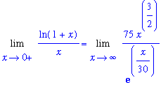


Example 6: p. 413, # 48
Note: Count Your Blessings!
This example was originally the essay question. But, I decided that I felt the question is not quite adequately worded, I wanted to be sure you saw specific parts of this problem, and the problem is too long and slightly difficult. Also, I believe the current essay question will be more generally useful for you later in this course.
The first thing you should notice about this problem is that we are looking at the limit as
 ->
->
 of a sequence of
functions
. We will talk about sequences in much more detail in Chapter 10, but most of that discussion is about sequences of
numbers
. The functions used in this example are really functions of the index,
 , and the variable,
 :
:
| > |
F := (n,x) -> n^2*x*exp(-n*x):
f[n](x) = F(n,x);
|
 = n^2*x*exp(-x*n)](images/lab7139.gif)
(a)
The requested plot is
| > |
plot( [seq(F(n,x),n=1..6)], x=0..1,
legend=[seq(sprintf("n=%a",n),n=1..6)] );
|
![[Maple Plot]](images/lab7140.gif)
(b)
To answer this question we should look at later terms in the sequence. Here are
![f[11]](images/lab7141.gif) , ..,
, ..,
![f[16]](images/lab7142.gif) .
.
| > |
plot( [seq(F(n,x),n=11..16)], x=0..1,
legend=[seq(sprintf("n=%a",n),n=11..16)] );
|
![[Maple Plot]](images/lab7143.gif)
Note that these functions have the same general shape but the maximum of each curve occurs earlier and is higher than for earlier curves in the sequence. For these functions, the function values are all very close to zero for all
 > 1/2.
Looking at the graph of
![f[51]](images/lab7145.gif) , ..,
, ..,
![f[56]](images/lab7146.gif) :
:
| > |
plot( [seq(F(n,x),n=51..56)], x=0..1,
legend=[seq(sprintf("n=%a",n),n=51..56)] );
|
![[Maple Plot]](images/lab7147.gif)
we see that this trend continues and that the functions appear to be essentially zero for all
 > 0.2.
For our final plot, let's look at
![f[1]](images/lab7149.gif) ,
,
![f[51]](images/lab7150.gif) ,
,
![f[101]](images/lab7151.gif) , and
, and
![f[501]](images/lab7152.gif) .
.
| > |
plot( [seq(F(n,x),n=[1,51,101,501])], x=0..1,
legend=[seq(sprintf("n=%a",n),n=[1,51,101,501])] );
|
![[Maple Plot]](images/lab7153.gif)
It is now pretty clear that, for each
 in [0,1]
,n = infinity) = 0](images/lab7155.gif) .
.
(c)
The six requested integrals are
| > |
for n from 1 to 6 do
q := Int( F(n,x), x=0..1 );
print( q=value( q ));
end do:
|


(d)
The results in (c) follow an obvious pattern:
,x = 0 .. 1) = -(n+1)*exp(-n)+1](images/lab7162.gif)
| > |
plot( [seq([n,Int(F(n,x),x=0..1)],n=1..20)], style=point, view=[0..20,0..1.5] );
|
![[Maple Plot]](images/lab7163.gif)
Thus, using Lab Question 6 (with
 and
and
 and with
 and
and
 ) we find
,x = 0 .. 1),n = infinity)](images/lab7168.gif) =
=
 =
=
 =
=
 = 1
= 1
Concluding Remarks
Observation 1:
,x = infinity)](images/lab7172.gif) and
and
,n = infinity)](images/lab7173.gif) are very different questions
are very different questions
For a
fixed index
,
 , Lab Question 6 (with
 and
and
 ) can be used to show
,x = infinity)](images/lab7177.gif) =
=
 =
=
 =
=
 = 0
= 0
But, this is a completely different question than looking at
,n = infinity)](images/lab7181.gif) for a
fixed value of the variable
,
for a
fixed value of the variable
,
 .
.
Observation 2: Interchanging limits is not always permitted
The real point of this example is to show that interchanging two limit operations may not be permissible. Here the two limits are the limit as
 ->
->
 and the limit involved in the Riemann Sum definition of the definite integral.
In (d) we found that
,x = 0 .. 1),n = infinity) = 1](images/lab7185.gif) .
.
Conversely, in (b), we found that for each specific value of x > 0:
,n = infinity) = 0](images/lab7186.gif) .
.
Therefore,
,n = infinity),x = 0 .. 1) = Int(0,x = 0 .. 1)](images/lab7187.gif) = 0.
= 0.
This means that
,x = 0 .. 1),n = infinity) <> Int(Limit(f[n](x),n = infinity),x = 0 .. 1)](images/lab7188.gif)
Lab Questions
1. p. 407, # 8
2. p. 408, # 32
3. p. 413, # 2
4

5

6. [Essay Question] Explain the steps needed to show that
 for all real values of
 >= 0 and all real values of
 > 0
> 0
Include how you rewrite the limit in an indeterminate form suitable to apply l'Hopital's rule and how many times l'Hopital's rule is applied. (Remember that
 and
and
 are real real numbers, not integers.) Also, explain how this limit justifies the following statement:
every exponentially growing function grows faster than every nonnegative power for large values of the variable.
 (p. 407, # 4)

![]() , it is difficult to know where to start. Most people just do not have the familiarity with the inverse trigonometric functions to be able to "see" the value of this limit. To begin to understand the problem, plot the function
, it is difficult to know where to start. Most people just do not have the familiarity with the inverse trigonometric functions to be able to "see" the value of this limit. To begin to understand the problem, plot the function
 on an interval containing the origin. Because the arcsin function is defined only on
![]() , that is the largest domain on which this function is defined.
, that is the largest domain on which this function is defined.
![[Maple Plot]](images/lab76.gif)
![]() ->0:
->0:
![]()
![]()
![]() , l'Hopital's rule can be applied. The derivatives of the numerator and denominator are
, l'Hopital's rule can be applied. The derivatives of the numerator and denominator are


![]()
![[Maple Plot]](images/lab718.gif)
![]() .
.

![[Maple Plot]](images/lab723.gif)
 (
(
 (
(
 . To verify that l'Hopital's rule applies


![[Maple Plot]](images/lab745.gif)
 (
(

![[Maple Plot]](images/lab753.gif)
 =
=
 =
=

 =
=
 =
=
 .
.

 =
=
 =
=
 =
=
 =
=

![[Maple Plot]](images/lab776.gif)
 =
=
 =
=
 .
.


 =
=
 =
=

![[Maple Plot]](images/lab798.gif)
![[Maple Plot]](images/lab799.gif)
![[Maple Plot]](images/lab7101.gif)
 .
.


![[Maple Plot]](images/lab7112.gif)


![[Maple Plot]](images/lab7120.gif)


![[Maple Plot]](images/lab7128.gif)


![[Maple Plot]](images/lab7140.gif)
![[Maple Plot]](images/lab7143.gif)
![[Maple Plot]](images/lab7147.gif)
![[Maple Plot]](images/lab7153.gif)
,n = infinity) = 0](images/lab7155.gif) .
.


,x = 0 .. 1) = -(n+1)*exp(-n)+1](images/lab7162.gif)
![[Maple Plot]](images/lab7163.gif)
,x = 0 .. 1),n = infinity)](images/lab7168.gif) =
=
 =
=
 =
=
,x = infinity)](images/lab7172.gif) and
and
,n = infinity)](images/lab7173.gif) are very different questions
are very different questions
,x = infinity)](images/lab7177.gif) =
=
 =
=
 =
=
,n = infinity)](images/lab7181.gif) for a
fixed value of the variable
,
for a
fixed value of the variable
,
,x = 0 .. 1),n = infinity) = 1](images/lab7185.gif) .
.
,n = infinity) = 0](images/lab7186.gif) .
.
,n = infinity),x = 0 .. 1) = Int(0,x = 0 .. 1)](images/lab7187.gif) = 0.
= 0.
,x = 0 .. 1),n = infinity) <> Int(Limit(f[n](x),n = infinity),x = 0 .. 1)](images/lab7188.gif)


 for all real values of