lab14.html

>

lab14.mws --- Numerical Evaluation of Series

> restart;
with( plots ):

Warning, the name changecoords has been redefined

>

Lab Overview

The typical textbook problem with series asks you to determine if a specific series converges or diverges. Rarely are you asked to find (even approximately) the sum of a convergent series. This lab is designed to fill this gap. You will approximate the sum of convergent series and see some of the different ways a series can fail to converge. For the Lab Questions you will be asked to analyze 4 series. For extra credit, you are asked to explain how rearranging the terms in the alternating harmonic series can change the sum of the series. If you pay attention to the presentation in lab on Tuesday, you should see how this can be done.

Continuing the practice from recent weeks, this lab assignment includes a separate and explicit integration problem. In fact, this week there are two integrals for a total of 4 points. You are encouraged to use the Integration maplet [ Maplet Viewer][ MapleNet] to help with this problem.

Deadline for submitting a lab solution is midnight, Thursday, April 24, 2003.

>

Example 1:

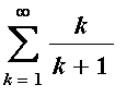
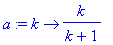
The terms in this series are . If this is entered as a Maple function, using

> a := k -> k/(k+1);

then the th partial sum can be defined to be

> s := n -> add( a(k), k=1..n );

For example, the first 10 terms in the series are

> terms := [seq([k,a(k)], k=1..10)]:
convert( terms, matrix );

and the corresponding partial sums for this series are

> partial_sums := [seq([k,s(k)], k=1..10)]:
convert( partial_sums, matrix );

To see these values as floating point numbers, use evalf :

> convert( evalf( terms ), matrix ),

> convert( evalf( partial_sums ), matrix );

The relationship between the sequences of terms and partial sums should be viewed graphically:

>    plot( [ terms, partial_sums ],
      style=point, color=[green,red],
      legend=["a[k] - term", "s[k] - partial sum"] );

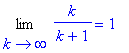
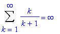
Notice how the terms (in green) level off around 1 and the partial sums increase (by about 1). Because the terms do not converge to zero, this series diverges by the th Term Test.

>

> L := Limit( a(k), k=infinity ):
L = value( L );

> S := Sum( a(k), k=1..infinity ):
S = value( S );

>

Example 2:

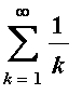
The terms in the harmonic series are . If this is entered as a Maple function, using

> a := k -> 1/k;

then the th partial sum can be defined to be

> s := n -> add( a(k), k=1..n );

For example, the first 10 terms in the series are

> terms := [seq([k,a(k)], k=1..10)]:
convert( terms, matrix );

and the corresponding partial sums for this series are

> partial_sums := [seq([k,s(k)], k=1..10)]:
convert( partial_sums, matrix );

To see these values as floating point numbers, use evalf :

> convert( evalf( terms ), matrix ),

> convert( evalf( partial_sums ), matrix );

The relationship between the sequences of terms and partial sums should be viewed graphically:

>    plot( [ terms, partial_sums ],
      style=point, color=[green,red],
      legend=["a[k] - term", "s[k] - partial sum"] );

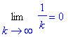
It is clear that the terms of this series converge to zero:

> L := Limit( a(k), k=infinity ):
L = value( L );

While the partials sums are increasing, it appears as though they might be leveling off. If so, then the series converges; if not, then the series diverges. Maybe we can answer this quesiton by looking at additional terms in the sequence of partial sums:

> partial_sum2 := [ seq([k,s(k)], k = [ 10*($1..10), 200*($1..4), 1000*($1..10)]) ]:
convert( evalf(partial_sum2), matrix );

> plot( evalf(partial_sum2), style=point );

The partial sums with up to 10,000 terms do not provide an answer to the question. The partial sums are still increasing but VERY slowly. Until we determine what happens with these partial sums we cannot decide if this series converges.

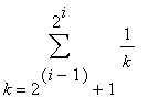
Of course, you have previously learned that the harmonic series. The typical explanation is that it is always possible to group the terms so that each group sums to at least 1/2. For example,

>    for i from 1 to 10 do
  lo := 1+2^(i-1);
  hi := 2^i;
  print( Sum( a(k), k=lo..hi ) = evalf(add( a(k), k=lo..hi )) )
end do:

In general, for any integer , the sum of the terms beginning with must be at least :

Because of this it is always possible to increase the partial sum by . This would not be possible if the harmonic series converged.

> S := Sum( a(k), k=1..infinity ):
S = value( S );

>

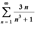
Example 3:

Note : This is #5d from Exam 3.

The terms in this series are . If this is entered as a Maple function, using

> a := n -> 3*n/(n^3+1);

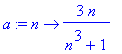
then the th partial sum can be defined to be

> s := n -> add( a(k), k=1..n );

For example, the first 10 terms in the series are

> terms := [seq([k,a(k)], k=1..10)]:
convert( terms, matrix );

and the corresponding partial sums for this series are

> partial_sums := [seq([k,s(k)], k=1..10)]:
convert( partial_sums, matrix );

To see these values as floating point numbers, use evalf :

> convert( evalf( terms ), matrix ),
convert( evalf( partial_sums ), matrix );

The relationship between the sequences of terms and partial sums should be viewed graphically:

>    plot( [ terms, partial_sums ],
      style=point, color=[green,red],
      legend=["a[k] - term", "s[k] - partial sum"] );

Notice how the terms (in green) converge to 0.

> L := Limit( a(n), n=infinity ):
L = value( L );

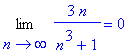
The partial sums increase and appear to level off. Based on our experience with the harmonic series, we know to be somewhat skeptical of "apparent leveling off". Instead of looking at additional partial sums - which will never provide a conclusive decision concerning the convergence or divergence of a series - let's try to use some of the convergence tests for series with positive terms.

>

Integral Test

The plot of the first 10 terms of the series suggests that these terms are monotonically decreasing to zero. The fact that the terms form a decreasing sequence can be confirmed by noting that

> Diff( a(x),x ) = simplify(diff( a(x), x ));

which is negative for all > 1. Thus, the Integral Test can be applied.

>

The improper integral

> q1 := Int( a(x), x=1..infinity ):
q1;

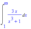
is difficult to evaluate by hand. (Note that = = so an antiderivative can be found using partial fractions with two terms. The details of this calculation will be omitted -- until you do it for Extra Credit.) Maple can evaluate this integral without difficulty:

> q1 = value( q1 );

Because this improper integral is finite, the series converges by the Integral Test.

>

Limit Comparison Test

Another method to determine the convergence of this series is the Limit Comparison Test. Observe that the highest degree term in the numerator is and the highest degree term in the denominator is . This suggests using = in the Limit Comparison Test.

> b := n -> 3/n^2:

To confirm that this is a valid choice of a comparison series, note that

> LCT_Limit := Limit( a(n)/b(n), n=infinity ):
LCT_Limit = value(LCT_Limit);

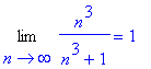
Now, because the series is a convergent -series with > 1, both series must converge.

>

Approximating the Sum of the Series

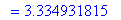
Now that we know the series converges, the question is: What is the sum of this series? Maple will tell us that

> S := Sum( a(n), n=1..infinity ):
S = value( S );
`` = evalf( S );

>

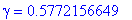
The exact formula requires some explanation:

is Euler's constant and is approximately

> gamma = evalf( gamma );

, the imaginary unit , and
is the digamma function (a special function defined by a complicated formula; you don't need - and probably don't care - to know more about this function!).

The floating point approximation is not difficult to understand. Because the terms are all positive, each parial sum will be less than -- and converging to -- the sum of the series. To conclude, we will determine the number of terms needed to approximate the sum of this series to 2 decimal places

>    for N from 0 do
  k := 2^N:
  app := evalf( s(k) ):
  err := evalf( S - app ):
  print( nprintf( "S[%5d] = %8.5f, Error = %8.5f", k, app, err ) );
  if err<0.005 then break end if;
end do:

That is, somewhere between 512 and 1024 terms are needed to approximate this integral to 2 decimal places. To narrow this range, repeat the above loop starting with the partial sum with 512 terms. (Repeating this process several times should lead you to the conclusion that 600 terms are needed to approximate the sum to 2 decimal places.)

>

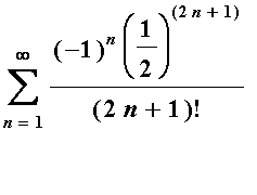
Example 4:

Note : This is the corrected version of #5e from Exam 3.

The terms in this alternating series are where . If this is entered as a Maple function, using

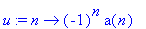
> u := n -> (-1)^n*a(n);
a := n -> (1/2)^(2*n+1)/(2*n+1)!;

then the nth partial sum can be defined to be

> s := n -> add( u(k), k=0..n );

For example, the first 11 terms in the series are

> pos_terms := [seq([k,a(k)], k=0..10)]:
terms := [seq([k,u(k)], k=0..10)]:
convert( terms, matrix );

and the corresponding partial sums for this series are

> partial_sums := [seq([k,s(k)], k=1..10)]:
convert( partial_sums, matrix );

To see these values as floating point numbers, use evalf :

> convert( evalf( terms ), matrix ),
convert( evalf( partial_sums ), matrix );

The relationship between the sequences of terms and partial sums should be viewed graphically:

>    plot( [ terms, partial_sums ],
      style=point, color=[green,red],
      legend=["u[k] - term", "s[k] - partial sum"] );

Notice how the terms (in green) immediately decay to a level where they become lost in the horizontal axis and the partial sums appear to be essentially constant with a value slightly smaller than -0.02. While these are strong indications that this series converges, the Alternating Series Test should be used.

Alternating Series Test

The Alternating Series Test applies only when the sequence of positive terms, , must be decreasing and converge to zero. The limit is easy to determine: positive integer powers of converge to zero and the factorial grows without bound.

> L_pos := Limit( a(n), n=infinity ):
L_pos = value(L_pos);

To see that the terms are decreasing for all positive integers ( >= 1), observe that

Now, the Alternating Series Test tells us that this series converges.

>

Ratio Test

From the analysis that the sequence of absolute values, a[n], is decreasing, we compute

= 0.

Because = 0 < 1, the Ratio Test tells us that the series converges absolutely.

>

Approximating the Sum of the Series

As with Example 3, knowing that the series converges we want to know an accurate approximation to the sum of the series. Maple will tell us that

> S := Sum( u(n), n=0..infinity ):
S = value( S );
`` = evalf( S );

>

This exact value should not be a complete surprise. Note that this series has only odd terms and the general form is that of with .

The floating point approximation is not difficult to understand. The method introduced in Example 3 can be used here with one modification. Because the series contains both positive and negative terms, the partial sums could be larger or smaller than the exact sum. An absolute value will take care of this. To determine the number of terms needed to approximate the sum of this series to 8 decimal places

>    Digits := 20:
for N from 0 do
  k := 2^N:
  app := evalf( s(k) ):
  err := evalf( abs(S - app) ):
  print( nprintf( "S[%5d] = %14.11f, Error = %14.11f", k, app, err ) );
  if err<0.000000005 then break end if;
end do:
Digits := 10:

Wow! This series converges so fast that the partial sum with 4 terms provides an estimate that is accurate to 8 decimal places.

>

In fact, because this series is an alternating series, the Alternating Series Test tells us that the partial sum with terms differs from the exact sum by no more than the next term in the series: . This suggests considering the equation

> eqn := a(n+1)=0.000000005;

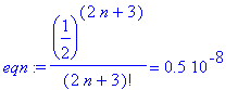
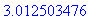
The solution to this equation is

> solve( eqn, n );

Recalling that must be an integer, round up to obtain , in agreement with the previous search.

Note how the additional information provided by the Alternating Series Test provides a much more efficient method for finding the number of terms needed to approximate a series with a prescribed accuracy.

>

Lab Questions

For each of the following series, explain why the series converges. For #1, #3, and #4:

i) approximate the series to 3 decimal places

ii) determine the number of terms needed to obtain the estimate in i)

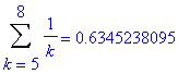
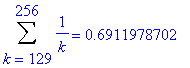
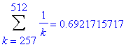
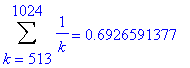
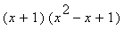
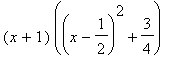
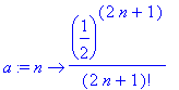
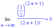
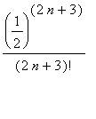
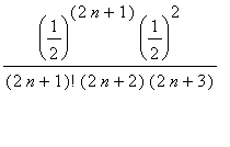
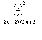
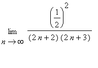
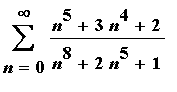
1. [2 pts]

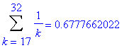
2. [2 pts]

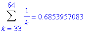
3. [2 pts]

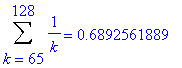
4. [2 pts]

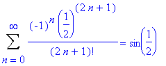
5. [Extra Credit: 2pts]

Explain how the terms in the alternating harmonic series can be rearranged so the sequence of partial sums converges to . Give the first 25 terms in the rearranged series.

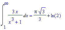
6. [Integration Problem: 2 pts]

Show all steps in the evaluation of the indefinite integral 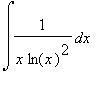= . You may use any technology to help solve this problem. Your answer, however, must explain all steps in the evaluation.

7. [Integration Problem: 2 pts]

Show all steps in the evaluation of the indefinite integral 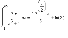. You may use any technology to help solve this problem. Your answer, however, must explain all steps in the evaluation.

>