lab13.mws --- Geometric Series and Drug Concentrations
| > |
restart;
with( plots ):
|
Warning, the name changecoords has been redefined
Lab Overview
This lab introduces and explores a pharmaceutical problem that is best addressed with mathematics. When we take (or are given) medication, the concentration of the drug in the bloodstream is not constant. The drug is effective when the concentration is above a certain threshold. Oftentimes there is also an upper limit on the concentration above which the drug becomes toxic. Two different models will be formulated. You know all the mathematics needed to model the drug concentration. For the Lab Questions, you will be asked to use these models to design a drug treatment regimin meeting specified constraints.
Continuing the practice started two weeks ago, this lab assignment includes a separate and explicit integration problem. You are encouraged to use the
Integration
maplet [
Maplet Viewer][
MapleNet] to help with this problem.
Deadline for submitting a lab solution is midnight, Thursday, April 17, 2003.
Problem Description
The concentration in the blood resulting from a single dose of a drug normally decreases with time as the drug is eliminated from the body. In order to determine the exact pattern the decrease follows, experiments are performed in which drug concentrations in the blood are measured at various times after the drug is administered. The data are then checked against a hypothesized function relating drug concentration to time.
We make a simplifying assumption: when the drug is administered, it is diffused so rapidly throughout the bloodstream that, for all practical purposes it reaches its fullest concentration instantaneously. This assumption is justified for drugs that are administered intravenously, for example, but certainly not for drugs that are taken orally.
Data for Two Drugs
We will consider two drugs, Drug A and Drug B. Suppose experiments with Drug A show that when the initial concentration is 1.0 mg/ml (millgram per milliliter) initially (
 ) and 0.15 mg/ml six hours later (
 ). This data will be represented in Maple as
| > |
dataA1 := [ t=0.0, C=1.0 ]:
dataA2 := [ t=6.0, C=0.15 ]:
|
The same experiment with Drug B shows the concentration drops from 1.5 mg/ml to 0.75 mg/ml over the same time period.
| > |
dataB1 := [ t=0.0, C=1.7 ]:
dataB2 := [ t=6.0, C=0.75 ]:
|
Two Different Models
Two different models for how the concentration changes as a function of time will be considered.
Model 1 - Constant Rate of Consumption
Assume the concentration of the drug in the blood is a linear function of the time since the first dose was administered.
Model 2 - Proportional Rate of Consumption
Assume the concentration of the drug in the blood decreases at a rate proportional to the current concentration in the blood.
Typical Questions of Interest
Each model will be explained and analyzed in subsequent sections of this worksheet. Some of the questions to be addressed include:
-
how does the drug concentration change over time? (this can be addressed with a graph)
-
predict the time when the blood becomes free of the drug (assuming no further doses are given)
-
suppose the drug is readministered every 6 hours for 2 days, graph the drug concentration against time for 48 hours
-
what happens if the drug is readministered every 6 hours indefinitely?
(in particular, what are the maximum and minimum concentrations that occur between doses?)
The question about maximum and minimum concentrations in the blood is particularly important to a physician. For most drugs, there is a concentration below which the drug is ineffective and another concentration above which the drug is dangerous. For example, suppose Drug B is ineffective below 0.45 mg/ml and the maximum safe level is 2.15 mg/ml. If the dose is repeated every 6 hours, will the appropriate concentrations be maintained? If so, for how long? What happens to the maximum and minimum concentrations over time?
In hospitals, where nurses generally administer medications, it is not possible to individually adjust the time interval between dosages. Realistically, the time interval will be every 4, 6, 8, or 12 hours. Can the dosage level be adjusted so that the concentration stays within the effective limits listed above?
Model 1: Constant Rate of Consumption
The rate at which the drug is removed from the blood is the derivative of the concentration:
 . If this rate is constant, then the concentration has a constant slope. Hence, the concentration must be a linear function of time.
| > |
model1 := C = m*t + b:
model1;
|

The two pieces of information for Drug A can be used to obtain 2 equations for the 2 unknown parameters in the model: the slope
 and the "intercept"
 :
:
![[t = 0., C = 1.0]](images/lab137.gif)
![[t = 6.0, C = .15]](images/lab138.gif)
| > |
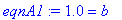
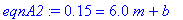
eqnA1 := eval( model1, dataA1 );
eqnA2 := eval( model1, dataA2 );
|
The solution to these two equations is
| > |
q1 := solve( { eqnA1, eqnA2 }, { m, b } );
|

Notice that the "intercept" is better described as the dosage amount. This is the amount of increase in the concentration when a dose of Drug A is given.
| > |
if not assigned(m) then assign( q1 ) end if;
dosage_amt := b;
dose_beg[1] := dosage_amt;
dose[1] := rhs(model1):
C = dose[1];
|

![dose_beg[1] := 1.](images/lab1313.gif)
The graph of this concentration as a function of time is the straight line in the following plot.
| > |
plot( dose[1], t=0..10, title="One Dose of Drug A: Concentration vs. Time" );
|
![[Maple Plot]](images/lab1315.gif)
When is the drug completely removed from the blood?
Now, if the medication is readministered at the end of 6 hours, then the concentration at
 will be increased by the dosage amount (
 mg/ml) from its measured level at the end of the first treatment period (
 ).
).
| > |
t2 := 6;
dose_end[1] := eval( dose[1], t=6 );
dose_beg[2] := dose_end[1] + dosage_amt;
|

![dose_end[1] := .1499999998](images/lab1320.gif)
![dose_beg[2] := 1.150000000](images/lab1321.gif)
Then, over the next 6 hours, the concentration of the drug is a linear function with the same slope as during the first 6 hours. That is, after dose 2 is administered, the concentration is the linear function:
| > |
dose[2] := dose_beg[2] + m*(t-t2):
C = dose[2];
|

Verify that this linear function has the proper slope and satisfies the condition that the concentration at
 is
is
 mg/ml. Thus, the plot of the concentration over the first two treatment periods is
| > |
P1 := plot( dose[1], t=0..6 ):
P2 := plot( dose[2], t=6..12 ):
display( [P1,P2], view=[DEFAULT,0..2],
title="Model 1: Two Doses of Drug A\nConcentration vs. Time" );
|
![[Maple Plot]](images/lab1325.gif)
A third dose after 12 hours would be handled in the same way:
| > |
t3 := 12;
dose_end[2] := eval( dose[2], t=t3 );
dose_beg[3] := dose_end[2] + 1;
dose[3] := dose_beg[3] + m*(t-t3):
C = dose[3];
|

![dose_end[2] := .300000000](images/lab1327.gif)
![dose_beg[3] := 1.300000000](images/lab1328.gif)

| > |
P3 := plot( dose[3], t=12..18 ):
display( [P1,P2,P3], view=[DEFAULT,0..2],
title="Model 1: Three Doses of Drug A\nConcentration vs. Time" );
|
![[Maple Plot]](images/lab1330.gif)
| > |
dose_end[3] := eval( dose[3], t=18 );
|
![dose_end[3] := .449999999](images/lab1331.gif)
Do you see the patterns in the concentration as additional doses of Drug A are administered?
| > |
HEADER := < `Dose #` | `Conc (beg)` | `Conc (end)` | `Difference` >:
R1 := < 1 | dose_beg[1] | dose_end[1] | dose_beg[1]-dose_end[1] >:
R2 := < 2 | dose_beg[2] | dose_end[2] | dose_beg[2]-dose_end[2] >:
R3 := < 3 | dose_beg[3] | dose_end[3] | dose_beg[3]-dose_end[3] >:
R4 := < 4 | `` | `` | `` >:
R5 := < 5 | `` | `` | `` >:
R6 := < 6 | `` | `` | `` >:
R7 := < 7 | `` | `` | `` >:
R8 := < 8 | `` | `` | `` >:
Model1_Table := < HEADER, R1, R2, R3, R4, R5, R6, R7, R8 >;
|
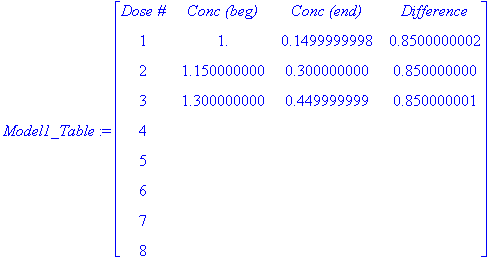
-
What is the drug concentration immediately before doses 4 and 8 of Drug A are administered?
-
What is the drug concentration of Drug A after 24 and 48 hours?
-
How long does a trace of the drug stay in the blood?
-
What would happen if the drug were administered for a full week?
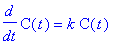
Model 2: Proportional Rate of Consumption
As above, let
 denote the concentration of the drug in the blood at time
 . Then the rate of change of the concentration,
 , is proportional to the concentration if
| > |
unassign( 'c','k' );
ode2 := diff( C(t), t ) = k*C(t):
ode2;
|
This differential equation is separable and can be solved by the methods discussed in Math 141 (see Section 5.2 of Varberg, Purcell, and Rigdon). The solution to this differential equation with initial condition

is
| > |
q2 := dsolve( {ode2,ic2}, C(t) ):
model2 := C = rhs(q2):
model2;
|

As for Model 1, the experimental data for Drug A can be used to find two equations from which the parameters
 and
and
 can be determined. Recall that the data points are
![[t = 0., C = 1.0]](images/lab1341.gif)
![[t = 6.0, C = .15]](images/lab1342.gif)
The corresponding two equations for
 and
and
 are
are
| > |
eqnA3 := eval( model2, dataA1 );
eqnA4 := eval( model2, dataA2 );
|
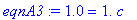
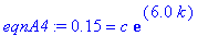
The solution to these equations is
| > |
q3 := solve( {eqnA3,eqnA4}, {c,k} ):
q3;
|

Observe that coefficient of the exponential function is the concentration of the drug immediately after the drug enters the bloodstream. The dosage amount is the coefficient of the exponential function
for the initial treatment period
. Thus, after one dose of Drug A, the concentration in the blood is
| > |
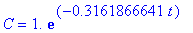
if not assigned(`k`) then assign( q3 ) end if;
t1 := 0;
dosage_amt := c;
dose_beg[1] := dosage_amt;
dose[1] := dose_beg[1] * exp( k*(t-t1) ):
C = dose[1];
|

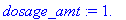
![dose_beg[1] := 1.](images/lab1350.gif)
| > |
plot( dose[1], t=0..24, title="Model 2: One Dose of Drug A\nConcentration vs. Time" );
|
![[Maple Plot]](images/lab1352.gif)
Notice that because the concentration follows an exponential curve, the drug is never completely removed from the blood.
If the medication is readministered at the end of 6 hours, then the concentration at
 will be increased by the dosage amount (
 mg/ml) from its measured level at the end of the first treatment period.
| > |
t2 := 6;
dose_end[1] := eval( dose[1], t=6 );
dose_beg[2] := dose_end[1] + dosage_amt;
|

![dose_end[1] := .1500000000](images/lab1356.gif)
![dose_beg[2] := 1.150000000](images/lab1357.gif)
This is unchanged from Model 1. The difference for Model 2 is seen after dose 2 is administered. Now, the concentration follows an exponential curve with the same decay rate (
 ) but the coefficient is the concentration immediately after dose 2 enters the bloodstream.
| > |
dose[2] := dose_beg[2] * exp( k*(t-t2) );
|
![dose[2] := 1.150000000*exp(-.3161866641*t+1.897119985)](images/lab1359.gif)
The graph of the concentration of Drug A in the blood for 2 full treatment periods (12 hours) is shown below.
| > |
P1 := plot( dose[1], t=0..6 ):
P2 := plot( dose[2], t=6..12 ):
display( [P1,P2], view=[DEFAULT,0..2],
title="Model 2: Two Doses of Drug A\nConcentration vs. Time" );
|
![[Maple Plot]](images/lab1360.gif)
A third dose after 12 hours would be handled in the same way:
| > |
t3 := 12;
dose_end[2] := eval( dose[2], t=t3 );
dose_beg[3] := dose_end[2] + dosage_amt;
dose[3] := dose_beg[3] * exp( k*(t-t3) ):
C = dose[3];
|

![dose_end[2] := .1725000001](images/lab1362.gif)
![dose_beg[3] := 1.172500000](images/lab1363.gif)

| > |
P3 := plot( dose[3],t=12..18 ):
display( [P1,P2,P3], view=[DEFAULT,0..1.5],
title="Model 2: Three Doses of Drug A\nConcentration vs. Time" );
|
![[Maple Plot]](images/lab1365.gif)
| > |
t4 := 18;
dose_end[3] := eval( dose[3], t=t4 );
|

![dose_end[3] := .1758750000](images/lab1367.gif)
Continuing this pattern for 8 doses of Drug A will give the concentration of Drug A for a full 2 days (48 hours). To see the patterns for this model, consider the following table
| > |
HEAD := < `Dose #` | `Time` | `Conc (beg)` | `Conc (end)` | `Ratio (end/beg)` >:
R1 := < 1 | t1 | dose_beg[1] | dose_end[1] | dose_end[1]/dose_beg[1] >:
R2 := < 2 | t2 | dose_beg[2] | dose_end[2] | dose_end[2]/dose_beg[2] >:
R3 := < 3 | t3 | dose_beg[3] | dose_end[3] | dose_end[3]/dose_beg[3] >:
R4 := < 4 | 18 | `` | `` | `` >:
R5 := < 5 | 24 | `` | `` | `` >:
R6 := < 6 | 30 | `` | `` | `` >:
R7 := < 7 | 36 | `` | `` | `` >:
R8 := < 8 | 42 | `` | `` | `` >:
Model2_Table := < HEAD, R1, R2, R3, R4, R5, R6, R7, R8 >;
|
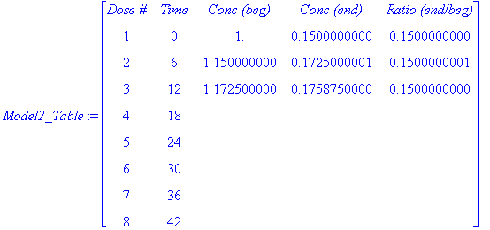
Notice the patterns in the the above table. Use these patterns to complete the remaining five rows of the table.
-
What is the drug concentration immediately before doses 4 and 8 of Drug A are administered?
-
What is the drug concentration of Drug A after 24 and 48 hours?
-
How long does a trace of the drug stay in the blood?
-
What would happen if the drug were administered for a full week?
General Analysis of Model 2
To understand exactly what is happening in Model 2, it is easier to work with the general model. Let
 denote the dosage amount (in mg/ml) for a single dose of the drug,
 be the decay rate for the concentration after it enters the bloodstream, and
 represents the time between treatments (the treatment period).
| > |
unassign( 'c', 'k', 'T' );
|
| > |
dosage_amt := c:
dose_beg[1] := dosage_amt:
dose[1] := dose_beg[1] * exp( k*t ):
for i from 2 to 8 do
t||i := (i-1)*T;
dose_end[i-1] := eval( dose[i-1], t=(i-1)*T);
dose_beg[i] := simplify( dose_end[i-1] + c );
dose[i] := simplify( dose_beg[i] * exp( k*(t-t||i) ) );
end do:
dose_end[i-1] := eval( dose[i-1], t=(i-1)*T ):
|
Concentration at Beginning of Treatment Cycles
The concentration of the drug in the blood at the beginning of the first few treatment periods is
| > |
for i from 1 to 8 do
printf( "Dose %a:", i );
print( dose_beg[i] );
end do;
unassign( 'i' );
|
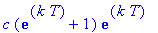
Dose 1:

Dose 2:
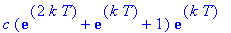
Dose 3:
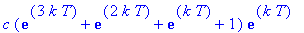
Dose 4:
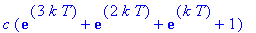
Dose 5:
Dose 6:

Dose 7:

Dose 8:

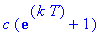
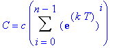
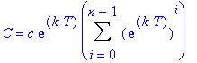
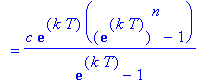
Observe that these expressions are successive partial sums of the geometric series with first term
 and radius
 . Thus, in general, the concentration of the drug in the blood at the beginning of treatment period n is
| > |
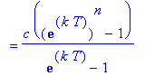
GenDoseBeg := c * Sum( exp(k*T)^i, i=0..(n-1) ):
C = GenDoseBeg;
`` = simplify(value( GenDoseBeg ));
|
Notice that for Drug A the radius
 = 0.15 (see
eqn2A
above).
= 0.15 (see
eqn2A
above).
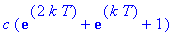
Concentration at End of Treatment Cycles
The concentration of the drug in the blood at the end of the first few treatment periods is
| > |
for i from 1 to 8 do
printf( "Dose %a:", i );
print( dose_end[i] );
end do;
unassign( 'i' );
|
Dose 1:

Dose 2:
Dose 3:
Dose 4:
Dose 5:

Dose 6:

Dose 7:

Dose 8:

Observe that these expressions are successive partial sums of the geometric series with first term
 and radius
 . Thus, in general, the concentration of the drug in the blood at the end of treatment period n is
| > |
GenDoseEnd := c*exp(k*T) * Sum( exp(k*T)^i, i=0..(n-1) ):
C = GenDoseEnd;
`` = simplify(value( GenDoseEnd ));
|
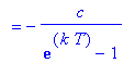
Notice that the concentrations at the beginning and end of the same treatment cycle are related by
| > |
C[`end`]/C[beg] = GenDoseEnd/GenDoseBeg;
|
![C[`end`]/C[beg] = exp(k*T)](images/lab1397.gif)
This provides another interpretation for the radius
 = 0.15 (see
eqn2A
above).
= 0.15 (see
eqn2A
above).
Extreme Values of Concentration
Analysis for Drug A
In the case of Drug A, we know
 and
and
 , and continue to use
 . These values of the parameters give the following general formulae for the concentratiosn at the beginning and end of treatment cycle n:
| > |
GenDoseBegA := eval( value( GenDoseBeg ), q3 union {T=6} ):
GenDoseEndA := eval( value( GenDoseEnd ), q3 union {T=6} ):
C[beg,n] = GenDoseBegA;
C[`end`,n] = GenDoseEndA;
|
![C[beg,n] = -1.176470588*.1500000000^n+1.176470588](images/lab13102.gif)
![C[`end`,n] = -.1764705882*.1500000000^n+.1764705882](images/lab13103.gif)
For the first eight doses, the concentrations immediately after the drug is administered are
| > |
seq( GenDoseBegA, n=1..8 );
seq( GenDoseEndA, n=1..8 );
|


-
Assuming Drug A is administered indefinitely every 6 hours, what is the highest concentration of Drug A in the blood?
-
What is the lowest concentration of Drug A?
-
At what times do these extreme concentrations occur?
General Analysis
During each treatment cycle the highest concentration occurs immediately after the drug is administered. With each successive treatment the initial amount increases. If the treatment continues indefinitely, the highest concentration is the value of the infinite geometric series
| > |
GenDoseMax := eval( GenDoseBeg, n=infinity ):
C[max] = GenDoseMax;
`` = value( GenDoseMax );
;
|
![C[max] = c*Sum(exp(k*T)^i,i = 0 .. infinity)](images/lab13106.gif)
During each treatment cycle the lowest concentration occurs at the end of the treatment cycle. These values increase from one treatment cycle to the next. Therefore, the lowest concentration occurs at the end of the first treatment cycle.
| > |
GenDoseMin := eval( GenDoseEnd, n=1 ):
C[min] = GenDoseMin;
`` = value( GenDoseMin );
;
|
![C[min] = c*exp(k*T)*Sum(exp(k*T)^i,i = 0 .. 0)](images/lab13108.gif)

Lab Questions
1. [2 pts]
Repeat the analysis of Model 1 for Drug B.
What is the slope of the graph of the concentration as a function of time?
Assuming Drug B is administered every 6 hours, what is the concentration at the end of a two-day treatment period?
2. [2 pts]
Repeat the analysis of Model 2 for Drug B.
What is the decay rate for the concentration?
Assuming Drug B is administered every 6 hours, what is the concentration at the end of a two-day treatment period?
3. [2 pts]
For Model 2 and Drug B, find a dosage amount
 so that the concentration of Drug B in the blood is between 0.45 mg/ml and 2.15 mg/ml for a treatment period that ends after two days.
4. [Essay Question: 1 pt]
Explain why, for Model 2, the formula for the minimum concentration
![C[min] = c*exp(k*T)](images/lab13111.gif) gives a value that is always less than the value given by the formula for the maximum concentration
gives a value that is always less than the value given by the formula for the maximum concentration
![C[max] = c/(1-exp(k*T))](images/lab13112.gif) .
.
Hint:
Use what you know about
 ,
,
 ,
,
 , and the exponential function.
5. [Integration Problem: 2 pts]
Show all steps in the evaluation of the integral
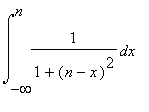 =
=
 . Note that this is similar -- but simpler -- than last week's integral. You may use any technology to help solve this problem. Your answer, however, must explain all steps in the evaluation.