DerivImplicit.html

Implicit Differentiation

> restart;
with( plots ):
with( Student[Calculus1] ):

Warning, the name changecoords has been redefined

>

Lesson Overview

Many interesting curves cannot be given in an explicit form

but can be given in implicit form

We know the slope of the tangent line to a curve at a point is and are now comfortable finding for explicit functions. Implicit differentiation is a technique that can be used to find when the function is given implicitly.

As this is really an application of the derivative, this lesson consists primarily of examples. The first example looks at a circle from both an explicit and an implicit formulation. The second example looks at a truly implicit function, the Folium of Descartes. The last example extends the Power Rule to all rational exponents.

The TangentLinePlot maplet [ Maplet Viewer][ MapleNet] can be used to assist with the visualization of tangent lines to the graph of an implicitly defined function.

>

Example 1: Tangent Lines for a Circle

The circle centered at the origin with radius 3 can be described as the set of all points that satisfy

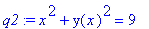
> q1 := x^2 + y^2 = 9:
q1;

Let be a number with -3 < < 3. Because both and are on the graph of the circle this is not a function.

> implicitplot( q1, x=-4..4, y=-4..4, title="The circle x^2+y^2=9" );

To find the slope of the tangent line to the circle at a point ( , ) on the circle, requires us to find . The idea behind implicit differentiation is to think of the equation of the circle implicitly defining as a function of . That means we need to replace all occurrences of y with y( ):

> yimpl := y=y(x):
yexpl := y(x)=y:
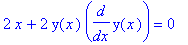
q2 := eval( q1, yimpl );

Now, if both sides of the equation are differentiated with respect to :

> q3 := diff( q2, x ):
q3;

Note the use of the Chain Rule to compute diff(y(x)^2,x) = 2*y(x)*diff(y(x),x) .

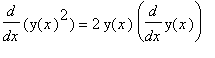It is now a simple matter to solve for the derivative

> q4 := isolate( q3, diff(y(x),x) ):
q4;

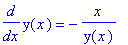
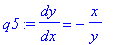
To put this result back in a form consistent with the original equation, replace all occurrences of with :

> q5 := dy/dx = eval( rhs(q4), yexpl );

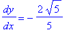
For example, the slope of the tangent line to this circle at the point ( 2, ) is

> eval( q5, [x=2,y=sqrt(5)] );

while at the point ( 2, ) the slope of the tangent line to the circle is

> eval( q5, [x=2,y=-sqrt(5)] );

What other methods could we use to find these slopes?

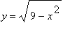
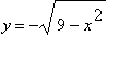
The top and bottom of the circle are, separately, graphs of functions:

> eq[top] := sqrt( 9 - x^2 ):
eq[bot] := -sqrt( 9 - x^2 ):
y[top] = eq[top];
y[bot] = eq[bot];

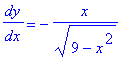
The slope at points on the top or bottom half of the plot can be found by differentiating these expressions. Unfortunately, we do not yet know how to differentiate the square root function. (At present the Power Rule only applies when the exponent is an integer.) But, letting Maple compute these derivatives for us, the slope of the tangent line at a point on the top half of the circle is found to be

> d1 := diff( eq[top], x ):
dy/dx = d1;

dy/dx = -1/(9-x^2)^(1/2)*x

The correctness of this result can be checked by using the general formula for the slope of the tangent line and the equation for the top of the circle:

> eval( q5, y=eq[top] );

dy/dx = -1/(9-x^2)^(1/2)*x

Likewise, the slope of the tangent line at a point on the bottom half of the circle is

> d2 := diff( eq[bot], x ):
dy/dx = d2;

dy/dx = 1/(9-x^2)^(1/2)*x

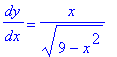
which agrees with the result from implicit differentiation:

> eval( q5, y=eq[bot] );

dy/dx = 1/(9-x^2)^(1/2)*x

>

The formula for obtained above is defined only if . This makes sense because when or and at these points the tangent lines are vertical. These features, together with the two tangent lines to the circle at points with , are evident in the following plot.

>    p1 := Tangent( eq[top], x=2, -4..4, output=plot,
               functionoptions=[color=red, legend=["Top of circle"]],
               tangentoptions=[color=gold,legend="Tangent to top of circle at x=2"] ):
p2 := Tangent( eq[bot], x=2, -4..4, output=plot,
               functionoptions=[color=blue, legend=["Bottom of circle"]],
               tangentoptions=[color=green,legend="Tangent to bottom of circle at x=2"] ):
display( [p1,p2], view=[-4..4,-4..4], title="The two tangent lines\n at x=2 for the circle\n x^2+y^2=9" );

[Maple Plot]

>

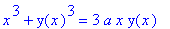
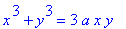
Example 2: Folium of Descartes

The general form for the Foliumm of Descartes is the implicit equation

> r1 := x^3 + y^3 = 3*a*x*y;

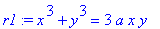
where is a parameter.

Visualizing the Folium of Descartes

Before analyzing these curves it will help to have an idea what these curves look like. The following animation shows plots of the Folium of Descartes for integer values of from -3 to 3.

>    Pfd := [seq( implicitplot( r1, x=-6..6, y=-6..6, numpoints=2000,
                           title=sprintf("Folium of Descartes: a=%a",a) ),
             a=-3..3 )]:

> display( Pfd, insequence=true );

For the Folium degenerates to the line . For all the curves are more interesting. In particular, there are regions where there are three points on the curve for a single value of . (This is to be expected because every cubic equation with real-valued coefficients has three real or complex roots --- and complex roots appear in conjugate pairs.)

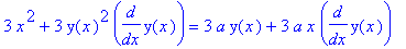
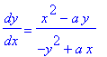
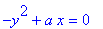
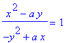
Finding Slope by Implicit Differentiation

Implicit differentiation will be used to find the slope of the tangent line at each point on the Folium of Descartes.

> r2 := eval( r1, yimpl ):
r2;

> r3 := diff( r2, x ):
r3;

> r4 := simplify(isolate( r3, diff(y(x),x) )):
r4;

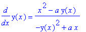
> r5 := dy/dx = eval(rhs(r4),yexpl):
r5;

Points on Curve with Horizontal Tangents

This information can be used to identify some special points on these curves. For example, the tangent line to the curve is horizontal at points on the curve where the slope is zero, i.e., points ( , ) that satisfy both

> r1;
r6 := numer( rhs(r5) ) = 0:
r6;

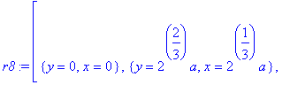
Maple reports the solutions to this pair of equations as

> r7 := [solve( {r1,r6}, {x,y} )];

$r7 := [{y = 0, x = 0}, {y = RootOf(_Z^3-2,label = _L1)^2*a, x = RootOf(_Z^3-2,label = _L1)*a}]$

The RootOf notation is Maple's way of concisely listing all real and complex roots of a polynomial. We can force the expansion to full solutions with the allvalues command:

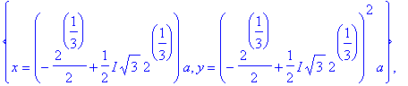
> r8 := map(allvalues,r7);

$r8 := [{y = 0, x = 0}, {y = 2^(2/3)*a, x = 2^(1/3)*a}, {x = (-1/2*2^(1/3)+1/2*I*3^(1/2)*2^(1/3))*a, y = (-1/2*2^(1/3)+1/2*I*3^(1/2)*2^(1/3))^2*a}, {y = (-1/2*2^(1/3)-1/2*I*3^(1/2)*2^(1/3))^2*a, x = (-1...$
$r8 := [{y = 0, x = 0}, {y = 2^(2/3)*a, x = 2^(1/3)*a}, {x = (-1/2*2^(1/3)+1/2*I*3^(1/2)*2^(1/3))*a, y = (-1/2*2^(1/3)+1/2*I*3^(1/2)*2^(1/3))^2*a}, {y = (-1/2*2^(1/3)-1/2*I*3^(1/2)*2^(1/3))^2*a, x = (-1...$
$r8 := [{y = 0, x = 0}, {y = 2^(2/3)*a, x = 2^(1/3)*a}, {x = (-1/2*2^(1/3)+1/2*I*3^(1/2)*2^(1/3))*a, y = (-1/2*2^(1/3)+1/2*I*3^(1/2)*2^(1/3))^2*a}, {y = (-1/2*2^(1/3)-1/2*I*3^(1/2)*2^(1/3))^2*a, x = (-1...$

Only the real-valued solutions are of interest to us so we remove all solutions that have an imaginary part:

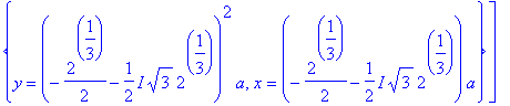
> r9 := remove( has, evalc(r8), I );

$r9 := [{y = 0, x = 0}, {y = 2^(2/3)*a, x = 2^(1/3)*a}]$

This leaves, for each value of , two points with horizontal tangents:

> seq( eval( [x,y], S ), S=r9 );

Points on Curve with Vertical Tangents

By the same reasoning, the slope of the tangent line to the curve is undefined at points that satisfy the two conditions

> r1;
r10 := denom(rhs(r5)) = 0:
r10;

The real-valued solutions to this system are found to be:

> r11 := [solve( {r1,r10}, {x,y} )]:

> r12 := map(allvalues,r11):

> r13 := remove( has, evalc(r12), I ):

> seq( eval( [x,y], S ), S=r13 );

Note that the origin has both a horizontal and a vertical tangent line and that the other points are symmetric about the line . (A closer look at the original equation and the formula for the slope explains why this - and other symmetries - are to be expected.).

Points on Curve with

Points where the slope of the tangent line is 1 are solutions to

> r1;
r14 := rhs(r5) = 1:
r14;

The real-valued solutions to this system are found to be:

> r15 := [solve( {r1,r14}, {x,y} )]:

> r16 := map(allvalues,r15):

> r17 := remove( has, evalc(r16), I ):

> seq( eval( [x,y], S ), S=r17 );

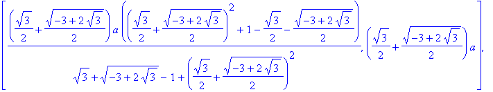
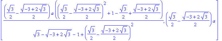
or, with floating-point approximations to the square roots

> seq( eval( [x,y], evalf(S) ), S=r17 );

Again, note the symmetry in these solutions. Note also that these solutions are not correct for . That there are no points on the graph with slope 1 when can be seen from the frame in the animation with as well as from Maple's response to the following command.

> [solve( eval( {r1,r14}, a=0 ), {x,y} )];

Concluding Comment: Explicit form for Folium of Descartes

At the beginning of this example it was implied that it is not possible to find an explicit representation for the Folium of Descartes. While it is true that each Folium is not the graph of a function, it is possible to find an explicit formula for each segment of the curve.

>    r18 := [solve( r1, {y} )]:
for S in r18 do
  print( "***********************************************************************" );
  op(S)
end do;

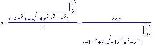
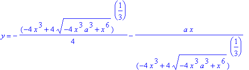
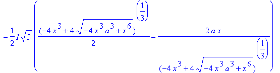
The first of the three solutions is always real-valued. The other two solutions are either real-valued or complex conjugates; when they are real-valued the Folium has three points for a single value of . and when they are complex conjugates there is only one point on the curve for each value of ; and at the transition between these states -- the unique value of with two point on the curve -- these two solutions reduce to a single repeated solution.

Even if we could decide which of these three formulae to use, the derivatives would be prohibitively complicated. By comparison, these computation by implicit differentiation was almost effortless.

>

Example 3: The Power Rule for Rational Exponents

In Example 1 we were unable to find the slope of the tangent line to a point on the top or bottom of a circle because we did not know how to differentiate the square root function. While we could have derived this result for the square root function using the definition of the derivative, it is much more efficient and useful to handle all rational exponents simultaneously. In this example implicit differentiation will be used to show the Power Rule applies for all rational exponents. That is, if with and integers and , then

The key is to convert the explicit form

> s1 := y = x^n:
s1;

to the implicit representation with integer exponents

> s2 := y^q = x^p:
s2;

To prepare for implicit differentiation, remind ourselves (and Maple) that :

> s3 := eval( s2, yimpl ):
s3;

Differentiation of both sides of the equation with respect to yields

> s4 := diff( s3, x ):
s4;

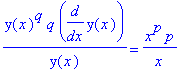
Thus,

> s5 := isolate( s4, diff( y(x), x ) ):
s6 := dy/dx = simplify( eval(rhs(s5),yexpl) ) assuming p::integer, q::integer;

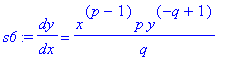
We would like to express this derivative explicitly in terms of . The explicit relationship with (so ) allow the derivative to be rewritten as

> qs := simplify( eval( s6, [s1,p=n*q] ) ) assuming q::integer:
qs;

This concludes the proof that the Power Rule applies for all rational exponents.

>

Lesson Summary

Given an implicitly defined function, , implicit differentiation is a technique for finding the slope of the tangent line to the curve, m = dy/dx . The key to successfully using implicit differentiation is to remember that one variable is implicitly defined in terms of the other, usually , and that differentiation of any term involving with respect to will automatically involve the Chain Rule.

An expression for obtained by implicit differentiation will typically involve both and . Examples 1 and 2 demonstrate how this form for the derivative can be used effectively. The final example extends the Power Rule from integer to rational exponents. Implicit differentiation will be used in the Related Rates lesson.

>

What's Next?

The online homework assignment includes a collection of practice problems that have been formulated to further your ability to successfully apply implicit differentiation. After you are comfortable with implicit differentiation, complete the textbook homework assignment related to this lesson.

After you finish all homework, and review the lessons in this unit, take Quiz 2 for Unit 2.

This concludes Unit 2. You now know all of the techniques needed to differentiate a large class of functions. You should also understand the connection between the derivative, (instantaneous) rates of change, and the slope of a tangent line to a curve. In Unit 3 the ideas introduced in this unit will be applied to a number of different applications.

>