An Overview of Maple 8
Introduction
Maple is a computer algebra system. While most mathematical software is restricted to working with numerical data, a computer algebra system is designed to perform symbolic manipulations of mathematical expressions. This document presents an overview of Maple with an emphasis on many of the features most likely to be of use in a first-year Calculus course.
Maple Arithmetic
At the simplest level, you can think of Maple as a powerful calculator that can do symbolic (exact) manipulations as well as floating point (approximate) numerical calculations.
Addition, Subtraction, Multiplication, and Division
The symbols
+, -, *, and /
are used for addition, subtraction, multiplication, and division, respectively. Don't try any of these on your graphing calculator!
| > |
575754575849849885 + 748949854985944749598984;
|
| > |
87575750 - 4897475988744894574949;
|
| > |
6868868686 * 18234987271740;
|
| > |
996868686127325465986865000000000000 / 5000;
|

Each command has to end with a
semi-colon
(or
colon
, if you don't wish to see the result).
Powers
Either
^
or
**
can be used to raise a number to a power.


Exponentials are handled with the
exp
command.

Euler's constant,
 , is obtained as

The Maple name for
 is
infinity
.
is
infinity
.

Palettes
Maple has three
palettes
containing shortcuts to entering commands via the keyboard. The
Expression
palette can be used to compute powers, roots, elementary transcendental functions, limits, derivatives, and other basic calculus-based quantities. To open this palette, pull down the
View
menu, choose
Palettes
and then select
Expression Palette
. Drag the palette to a position where it does not interfere with the current worksheet. (You may also need to resize the Maple and/or worksheet window.)
To use the palette to enter a quantity like
 , position the cursor in an empty input region,

click on the symbol
 in the palette. This produces
sqrt(
in the palette. This produces
sqrt(
 )
with the argument (
%?
) selected. Type
390625
and then execute the group. Your final input and output should appear as
)
with the argument (
%?
) selected. Type
390625
and then execute the group. Your final input and output should appear as

When a palette generates a template that involves more than one argument, the
Tab
key can be used to move from one argument to the next. For example, to compute
 , use the a / b button on the palette, enter 757555, press
Tab
, enter 5, then press
Return
to obtain
, use the a / b button on the palette, enter 757555, press
Tab
, enter 5, then press
Return
to obtain

Exact vs. Approximate Calculations
Maple is designed to provide exact answers to mathematical computations.

While the exact simplification in the previous example is useful, there are times when an exact answer is not helpful. For example, the following rational number is returned unchanged because it is already in reduced form.

There are several ways to instruct Maple to produce an approximate value for this number. Maple will display an answer as a floating point number if at least one number in the calculation is a floating point number (i.e., contains a decimal point).

The
evalf
command can also be used to force Maple to
eval
uate using
f
loating point arithmetic

By default, Maple performs all floating point computations using 10 significant digits. The following command performs the same calculation except that only 5 significant digits are used in the calculations. (See also the online help for
Digits
.)

Assigning Values to Names
Using Previous Results
The
ditto operator
%
always represents the result of the last command executed by Maple.

At this point, the most recent result computed is 5. This can be squared with the command

It is permissible to include more than one command in a single input region. For example,


In this case, the most recent result is -7. The next most recent result can recalled with
%%
.
Warning, incomplete quoted name; use ` to end the name
The ditto operators should be used sparingly. You should get in the habit of assigning results to explicit names.
Assignments
The Maple command for assigning a value to a name is the two-character sequence ``
:=
''. The single character ``
=
'' is used to form equations or to test for equality of two objects. Names generally consist of a letter followed by one or more letters, numbers, and underscores.
The commands to assign
x
the value 2 and
y
the value 3 are


The name
prod
will be assigned the product of
x
and
y

From now on, the name
prod
will be replaced with this value. Thus,

and, if the value of
x
is changed, the value of
prod
is not affected


The
unassign
command removes assignments to the listed names; note that the single quotes are required to prevent Maple from evaluating these names to their assigned values. (To erase
all
assignments, it is easier to use
restart;
.)
| > |
unassign( 'x', 'y', 'prod' );
|

Note that a different behavior is obtained if we define
prod
as before, but before assigning values to
x
and
y
,

When values are assigned to
x
and
y
, these values are used to compute the current value of
prod
.


And, if one or both of
x
and
y
are changed, the value of
prod
changes as well.


The difference in these two examples is whether the names used in the definition of
prod
have values
at the time the assignment is made
.
Suppressing Output
The last few examples have had more than one command in each input region. In this example, multiple names receive values in a single assignment. In this case the result of this assignment is suppressed because the assignment command is terminated with a colon.
| > |
x, y := 90, 30:
x; y; prod;
|


Maple Commands
Built-In Commands and Constants
Maple commands consist of a string of letters (and numbers) followed by one or more arguments enclosed in round brackets (parentheses). The
evalf
and
unassign
commands have already been encountered in this worksheet. Here are a few more examples.
If
 and
and
 are integers,
$
are integers,
$
 ..
..
 returns the list of all integers from
 to
to
 inclusive.

If
 represents a expression sequence of numbers, then
min(
represents a expression sequence of numbers, then
min(
 )
will return the smallest number in
)
will return the smallest number in
 .
.

To find the smallest number in a set or list, the surrounding brackets must be eliminated to obtain an expression sequence.
![L := [2, 3, 6]](images/maple8-overview56.gif)
Error, (in simpl/min) arguments must be of type algebraic

The following
plot
command will plot the function
 on the domain [
 ,
,
 ].
].
| > |
plot( cos(x) - x, x = -Pi .. 2*Pi );
|
![[Maple Plot]](images/maple8-overview61.gif)
In Maple, the equation
 is represented exactly as we would write it by hand. Note the use of
=
to form an equation, not the assignment operator
:=
. The following
fsolve
command locates a solution to
is represented exactly as we would write it by hand. Note the use of
=
to form an equation, not the assignment operator
:=
. The following
fsolve
command locates a solution to
 near
near
 .
.
| > |
fsolve( cos(x) - x = 0, x = 0 .. 2 );
|

As mentioned previously, some Maple names are predefined to standard constants. For example,
Pi
is
 . Recall that Euler's constant,
 , is obtained with
exp(1)
.
, is obtained with
exp(1)
.
| > |
evalf( Pi );
evalf( exp(1) );
|


| > |
evalf( Pi^exp(1) ) < evalf( exp(Pi) );
|
The command for the square root of a number
 is
sqrt(x)
.
is
sqrt(x)
.

Note that Maple has no trouble handling the square root of a negative number;
I
is the imaginary unit, i.e.,
 .
.

Each of these quantities could also have been assembled using the expresssion palette.
Command Options
Many Maple commands, particularly the plotting commands, accept optional arguments for customizing the output. For example, the option
linestyle=3
plots the command using a dashed line.
| > |
plot( sin(x) + cos(2*x), x = 0 .. 4*Pi, linestyle = 3 );
|
![[Maple Plot]](images/maple8-overview75.gif)
In the next
plot
command, two functions,
 and
and
 , are plotted simultaneously with the first function appearing as a dashed line and the second as a solid line. (Although it is not apparent in a hardcopy of this worksheet, Maple displays the first plot in red and the second in green. The
color=
option can be used to control the colors used in a plot.)
, are plotted simultaneously with the first function appearing as a dashed line and the second as a solid line. (Although it is not apparent in a hardcopy of this worksheet, Maple displays the first plot in red and the second in green. The
color=
option can be used to control the colors used in a plot.)
| > |
plot( [x^2, x^2*sin(x)^2], x = -5*Pi .. 5*Pi, linestyle = [ 1, 3 ] );
|
![[Maple Plot]](images/maple8-overview78.gif)
For a complete listing of the optional arguments for the
plot
command, see the online help for
plot,options
.
Online Help
The Maple command for accessing information in the online help database is
help(
 );
, or the abbreviated form
?
);
, or the abbreviated form
?
 . The help information appears in a separate window within Maple. While the help document appears to be very similar to a Maple worksheet, it is not possible to execute any commands that appear in a help document. Commands in the Examples section of a help worksheet can be copied individually or in their entirety and pasted in worksheet. To return to an active worksheet, either close the help window or select the desired window in the list of windows under the
Window
menu.
. The help information appears in a separate window within Maple. While the help document appears to be very similar to a Maple worksheet, it is not possible to execute any commands that appear in a help document. Commands in the Examples section of a help worksheet can be copied individually or in their entirety and pasted in worksheet. To return to an active worksheet, either close the help window or select the desired window in the list of windows under the
Window
menu.
The
Help
menu can also be used to browse the online help database. This is particularly powerful when you do not know the command name. The
New User's Tour
is particularly useful for new users.
Packages
In addition to the standard Maple functions available to you at the beginning of every Maple session, there are an ever-growing number of additional functions contained in
packages
that must be loaded into the Maple session prior to their use. The
with
command is used to load a package. Two of the more common packages for use in a Calculus course are the
plots
and
Student[Calculus1]
packages.
Warning, the name changecoords has been redefined


| > |
with( Student[Calculus1] );
|


The output of a successful
with
command is the list of commands that have been added to Maple's repertoire. If this list is unwanted, use a colon to terminate the command.
One of the commands that is now defined is
implicitplot
.
| > |
implicitplot( x^2 + y^4 = y^2 - x,
x = -1.3 .. 0.3, y = -1.2 .. 1.2,
scaling=constrained );
|
![[Maple Plot]](images/maple8-overview92.gif)
The
scaling=constrained
option instructs Maple to use the same scaling for each axis in the plot.
Creating Functions
Users can create their own Maple commands, including Maple implementations of mathematical functions. For example, the function
 can be defined using
| > |
f := x -> x^2 * sin(x)^2;
|
The variable
 is a dummy variable; it is replaced by whatever object appears as the first argument to
f
.
is a dummy variable; it is replaced by whatever object appears as the first argument to
f
.


Notice how Maple automatically simplifies the value of the function when possible.
To plot the function you can use either of the following commands
| > |
plot( f(x), x = -5*Pi .. 5*Pi );
|
![[Maple Plot]](images/maple8-overview99.gif)
| > |
plot( f, -5*Pi .. 5*Pi );
|
![[Maple Plot]](images/maple8-overview100.gif)
The plots are identical, except for the label on the horizontal axis.
The
unapply
command provides a second way to define a Maple function.
| > |
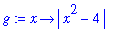
g := unapply( abs(x^2-4), x );
|
![[Maple Plot]](images/maple8-overview102.gif)
Notice that the output of the
unapply
command uses the same arrow notation as was used to define
f
above. The main difference between the arrow operator and
unapply
is that the argument to
unapply
is evaluated
before
the function is created. In contrast, the right-hand side of the arrow operator is
not evaluated
.
Lists and Sets
Definitions
Two of the most important data structures in Maple are the list and set. A
list
is an ordered expression sequence contained in square brackets,
[
 ]
, and a
set
is an unordered expression sequence contained in braces,
{
]
, and a
set
is an unordered expression sequence contained in braces,
{
 }
. (An
expression sequence
is a comma-separated collection of numbers, names, equations, or other Maple objects.)
}
. (An
expression sequence
is a comma-separated collection of numbers, names, equations, or other Maple objects.)
![L := [6, 7, 8, 9, 10]](images/maple8-overview106.gif)
Notice that the elements of a list or set can be any valid Maple object, including another list or set.
![SS := {{1, 3, 111}, [6, 7, 8, 9, 10]}](images/maple8-overview107.gif)
![LL := [[6, 7, 8, 9, 10], {1, 3, 111}]](images/maple8-overview108.gif)
Look carefully at the previous results. Even though the only difference in the definition of
LL
and
SS
is the type of brackets, the order of the elements in
SS
might appear in the opposite of the order in which they appeared in the definition. Recalling that the elements of a set are not ordered, this is not surprising. (It should also not be surprising to know that the order in which Maple displays the elements of a set can change from one session to another.)
Creating Lists and Sets
Except for the surrounding brackets, lists and sets are created in exactly the same ways. We have already seen how to create lists and sets from explicit collections of numbers and with the repetition command (
$
). The
seq
and
map
command provide two additional methods for creating lists and sets.
The
seq
command generates an expression sequence consisting of terms formed from the first argument for each value of the second argument. For example, the squares of the first ten positive integers is
| > |
pts := [ seq( i^2, i = 1 .. 10 ) ];
|
![pts := [1, 4, 9, 16, 25, 36, 49, 64, 81, 100]](images/maple8-overview109.gif)
This list could also be created using
$
as
![[1, 4, 9, 16, 25, 36, 49, 64, 81, 100]](images/maple8-overview110.gif)
To plot a list of
values
against their index in the set, use the
listplot
command from the
plots
package. The
style=point
optional argument instructs Maple to display discrete points (not connected),
symbol=cross
sets the plot symbol (the default is a diamond), and
symbolsize=20
sests the size of the symbols (in points; the default is 10).
| > |
listplot( pts, style=point, symbol=cross, symbolsize=20);
|
![[Maple Plot]](images/maple8-overview111.gif)
A list of 101
points
on the polar curve
 is constructed and displayed next. The list is not displayed as it is quite lengthy. Because the list elements include both the
 - and
- and
 -coordinates, the
plot
command can be used.
-coordinates, the
plot
command can be used.
| > |
rose4 := [ seq( [r(t*Pi/50)*cos(t*Pi/50), r(t*Pi/50)*sin(t*Pi/50)],
t = 0..100 ) ]:
|
![[Maple Plot]](images/maple8-overview115.gif)
The same plot could also have been created directly with any of the following variations of the
plot
command.
| > |
plot( [ r(t) * cos(t), r(t) * sin(t), t = 0 .. 2*Pi ] ):
|
| > |
plot( r(t), t = 0 .. 2*Pi, coords=polar ):
|
The last two commands show to create the graph of a parametric curve (C:
 ,
,
 for
for
 in
in
![[0, 2*Pi]](images/maple8-overview119.gif) ) and how to plot a polar function by specifying only the radius function and the range for the polar angle.
) and how to plot a polar function by specifying only the radius function and the range for the polar angle.
Extracting Elements of a List or Set
Much more than plotting can be done with a list or set. The third element of the list
pts
can be accessed as

Notice that it does not make sense to talk about the third element of a set. While Maple will not object to this, you should not expect to receive the same result every time the command is executed. The
select
and
remove
commands are designed to extract elements of a set that meet certain criteria. For example, the subset of
S
containing all elements that are in the open interval ( -10, 10 ) can be found as follows. (The
evalb
command returns either
 or
or
 (or
(or
 ) indicating the Boolean value of its argument.)

| > |
select( x -> evalb( abs( x - 10 ) < 20 ), S );
|

The number of elements in a list or set can be determined with the
nops
command.

Recall that each element of
rose4
is an ordered pair -- actually, a two-element list.
![[sin(9/25*Pi)*cos(9/50*Pi), sin(9/25*Pi)*sin(9/50*Pi)]](images/maple8-overview127.gif)
A floating-point approximation to this point is
![[.7639707480, .4848305795]](images/maple8-overview128.gif)
The
 -coordinate of the tenth element of the list is
Negative indices can be used to reference elements relative to the end of the list. The last point in
rose4
is
| > |
rose4[ -1 ] = rose4[ nops(rose4) ];
|
![[0, 0] = [0, 0]](images/maple8-overview131.gif)
The first ten elements of rose for can be specified using
rose4[ 1 .. 10 ]
. The floating point approximations to the
 -coordinates of each of these points can be obtained with
| > |
seq( evalf(p[1]), p = rose4[ 1 .. 10 ] );
|

Sets can also be manipulated using the standard set operators:
union
,
intersect
, and
minus
. Each of these commands can be used both as an infix operator, following standard mathematical notation, or as a prefix operator, which looks more program-like.
| > |
word := { "to", "too", "two" };
num := { "one", "two", "three", "four" };
|


The quotes on the command in the prefix form of the commands are required (to delay evaluation). The prefix forms of
union
and
intersect
can accept any number of sets.
Extracting Solutions to an Equation
When Maple finds the solution to an equation or system of equations, the output will be displayed as an expression sequence. You will often want to convert this to a list or set by inserting the appropriate brackets around the
solve
(or
fsolve
) command.
| > |
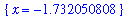
sol := [ fsolve( x^2 = 3, {x} ) ];
|
![sol := [{x = -1.732050808}, {x = 1.732050808}]](images/maple8-overview141.gif)
Approximations to the four solutions to the quartic polynomial equation
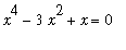 can be found, as a set, using
| > |
realsol := { fsolve( x^4 - 3*x^2 + x = 0, x ) };
|

In general,
fsolve
returns at most one (real) solution. For a polynomial, all real valued solutions are returned. To obtain complex-valued solution, add
complex
as an optional argument.
| > |
complexsol := { fsolve( x^4 - 3*x^2 + x = 4, x, complex ) };
|

Any individual solution can be obtained as above, but the result would depend on the order of the elements in a set -- which is unpredicable.

The largest element of a set can be found using

The absolute value of each solution can be obtained using
| > |
map( abs, complexsol );
|

To sort the four real roots in increasing order, re-express the solutions as a list and then call the
sort
command
| > |
realsol2 := convert( realsol, list );
|
![realsol2 := [-1.879385242, 1.532088886, .3472963553, 0.]](images/maple8-overview149.gif)
![[-1.879385242, 0., .3472963553, 1.532088886]](images/maple8-overview150.gif)
To sort the solutions by other orderings, e.g., the magnitude of the solutions, a user-defined ordering can be specified as the second argument to the
sort
command
| > |
sort( realsol2, (a,b) -> evalb( abs(a) < abs(b) ) );
|
![[0., .3472963553, 1.532088886, -1.879385242]](images/maple8-overview151.gif)
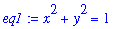
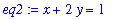
To conclude this discussion, consider the system of equations that describes the set of all points on the unit circle,
 , and the line,
 .
.
| > |
eq1 := x^2 + y^2 = 1;
eq2 := x + 2*y = 1;
|
The system of equations and variables are each specified as sets that, when fed to the
solve
command, show two solutions
| > |
syssol := [ solve( { eq1, eq2 }, { x, y } ) ];
|
![syssol := [{x = 1, y = 0}, {y = 4/5, x = -3/5}]](images/maple8-overview156.gif)
Each solution is a set of equations giving the
x
- and
y
-coordinates of a point on both curves. Note that the order of the equations within each solution may not be consistent. These solutions can be converted to ordered pairs using
| > |
syspts := seq( eval( [x,y], pt ), pt = syssol );
|
![syspts := [1, 0], [-3/5, 4/5]](images/maple8-overview157.gif)
The two curves involved in this problem can be plotted with the
implicitplot
command from the
plots
package. The two solutions can be plotted using
plot
with
style=point
. The
display
command (also from the
plots
package) can be used to display the information in both plots in a single plot. The output from the plot-creating commands in the definition of
p1
and
p2
is the corresponding ``plot data structure'', not a graphical object. (If you really want to see this, change the colons to semi-colons.)
| > |
p1 := implicitplot( { eq1, eq2 }, x = -2 .. 2, y = -2 .. 2,
scaling=constrained ):
p2 := plot( [ syspts ], style=point, color=black, symbol=circle,
symbolsize=30 ):
display( [ p1, p2 ] );
|
![[Maple Plot]](images/maple8-overview158.gif)
Note that the
implicitplot
command cannot accept a list as its first argument. This inconsistency with the other plot commands is corrected in Maple 9.
Creating Animations
A Maple animation is formed when the elements of a list of Maple plots is displayed in rapid succession. To animate the drawing of a function
 for 0 <
 <
<
 in polar coordinates, create a sequence of plots of the function over shorter time intervals, say 0 <
 <
<
![theta[0]](images/maple8-overview163.gif) for
for
![theta[0]](images/maple8-overview164.gif) =
=
 ,
,
 ,
,
 , ...,
 .
.
| > |
polarframes := seq( plot( sin(5*theta), theta = 0 .. theta0,
coords=polar ),
theta0 = [ n * Pi/12 $ n = 1 .. 12 ] ):
|
The
display
command from the
plots
package will display the plots as a list with the
insequence=true
option. The animation is, of course, playable only in an active Maple worksheet (or a worksheet that has been exported to HTML). To play the animation, click the left mouse button anywhere in the first frame of the animation. Then use the VCR control buttons on the context bar to advance through the frames individually, once from beginning to end, or continuously.
| > |
display( [ polarframes ], insequence=true );
|
![[Maple Plot]](images/maple8-overview169.gif)
For a hardcopy of this animation it makes more sense to display all 12 frames of the animation as an array (or matrix) with three rows each containing four plots. The
matrix
command, from the
linalg
package, is used to create the 3 x 4 array of plots, then the
display
command is used to display the result. The optional argument
tickmarks=[0,0]
suppresses the tickmarks on both axes (they become too cluttered to be of any use).
Warning, the protected names norm and trace have been redefined and unprotected
| > |
display( matrix( 3, 4, [polarframes]), tickmarks=[0,0] );
|
![[Maple Plot]](images/maple8-overview170.gif)
The concluding example in this section illustrates the relationship between the unit circle and the sine curve. The basic idea is to create separate plots of the sine curve and the unit circle centered at (-1,0). The animation comes with the addition of the line segment from the center of the circle to a point on the circle and the line segment from this point on the circle to the corresponding point on the sine curve for different angles between 0 and
 . Do not be concerned if some of the details are unclear at first. Once you see the animation and look at the individual pieces used to compose the individual frames, the process will become much less mysterious.
The unit circle with center (-1,0) can be created with the
circle
command from the
plottools
package.
Warning, the name arrow has been redefined
| > |
p1 := circle( [-1,0], 1, color=blue ):
|
| > |
p2 := plot( sin(x), x=0 .. 2*Pi, color=red ):
|
User-defined functions are used to create the line segments from the center of the circle, (-1,0), to a point on the circle, (
 -1,
-1,
 ), to the point on the sine curve, (
 ,
,
 ), for an arbitrary angle and the composite plot showing the circle, sine curve, and line segments..
| > |
circ_pt_line := t -> plot( [ [-1,0], [cos(t)-1,sin(t)], [t,sin(t)] ],
color=black ):
|
| > |
composite_plot := t -> display( [ p1, p2, circ_pt_line(t) ],
view=[-2..7,-1..1], tickmarks=[0,0],
scaling=constrained ):
|
The frame of the movie with
 can now be created with the command
| > |
composite_plot( Pi/4 );
|
![[Maple Plot]](images/maple8-overview177.gif)
The list of 32 uniformly distributed angles between 0 and
 is
is
| > |
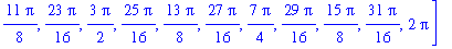
angles := [ i*Pi/16 $ i = 1 .. 32 ];
|

We conclude by making a frame for each of these angles and animating the resulting list of composite plots.
| > |
movieframes := [ seq( composite_plot( theta ), theta=angles ) ]:
|
| > |
display( movieframes, insequence=true, scaling=constrained );
|
![[Maple Plot]](images/maple8-overview181.gif)
Three Types of Brackets in Maple
Three types of brackets have been described in this worksheet:
( ... )
,
[ ... ]
, and
{ ... }
.
Parentheses or round brackets,
( ... )
, are used for the mathematical grouping of terms, including the specification of function arguments.


Square brackets,
[ ... ]
, are used for creating lists.
| > |
[ seq( n^2, n=-2..2 ) ];
|
![[4, 1, 0, 1, 4]](images/maple8-overview184.gif)
Curly brackets,
{ ... }
, are used for creating sets.
| > |
{ seq( n^2, n=-2..2 ) };
|

Do not attempt to interchange these symbols!
For example,
![sin[1/4*Pi]](images/maple8-overview186.gif)
Error, invalid input: exp expects its 1st argument, x, to be of type algebraic, but received {3}
Common Problems and How to Fix Them
Using a Command That Is Not Known by the Maple Kernel
Some commands are defined as part of a
package
that is not automatically loaded into the Maple kernel. If one of these commands is used prior to loading the package, the output will simply echo the input after the arguments have been simplified (if possible). For example,
| > |
completesquare( x^2 + 2*x + 2 );
|


| > |
completesquare( x^2 + 2*x + 2 );
|

Using Reserved Words and Protected Names
Maple places relatively few restrictions on the names that can be used for objects. When such a name is used, Maple generates an appropriate error message.
Error, reserved words `union` or `minus` unexpected
Error, attempting to assign to `Pi` which is protected
Be forewarned, however, that if a value is assigned to a name that is also a Maple command, then the new assignment overwrites the command definition. This feature can be used --- by knowledgeable and brave users --- to extend or customize the functionality of some of Maple's built-in commands.
Maple and Calculus
The techniques introduced in the earlier parts of this section will now be applied to the fundamental calculus concepts: limit, derivative, and integral and their applications.
Limits
The Maple command to compute
 is
limit
( f(x), x=a );
.
is
limit
( f(x), x=a );
.
| > |
limit( sin(x)/x, x=0 );
|

| > |
limit( (1+x)^(1/x), x=0 );
|

To obtain a limit at
 , use
infinity
.
, use
infinity
.
| > |
limit( (1+x/n)^n, n=infinity );
|

Right- or left-hand limits are returned when the (optional) third argument is
right
or
left
, respectively.
| > |
limit( tan(x), x=Pi/2 );
|

| > |
limit( tan(x), x=Pi/2, right );
|

| > |
limit( tan(x), x=Pi/2, left );
|

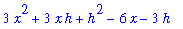
Derivatives and Tangent Lines
Given a function f, the slope of the secant lines through (
 ,
,
 ) and (
 ,
,
 ) is the difference quotient. As
 approaches 0, these quantities become the slope of the tangent line at (
 ,
,
 ). The slope of the secant line can be obtained with the Maple command
| > |
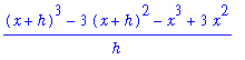
m[secant] := (f(x+h) - f(x) ) / h;
|
![m[secant] := (f(x+h)-f(x))/h](images/maple8-overview207.gif)
In practice, it is often necessary to use the simplify command to force Maple to
simplify
the difference quotient. For example,
| > |
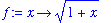
f := x -> x^3 - 3*x^2 - 4;
|
| > |
m[tangent] := limit( m[secant], h=0 );
|
![m[tangent] := 3*x^2-6*x](images/maple8-overview211.gif)
The
Tangent
command from the
Student[Calculus1]
package provides a simple means to display a function and the tangent line at a point.
| > |
with( Student[Calculus1] );
|


| > |
Tangent( f(x), x=1, output=plot );
|
![[Maple Plot]](images/maple8-overview217.gif)
The equation of this tangent line is obtained by changing the third argument to
output=line
.
| > |
Tangent( f(x), x=1, output=line );
|

The
TangentLinePlot
maplet [
MapletViewer] [
MapleNet] provides a customized user interface to the
Tangent
command. The
MapleNet version of this maplet is available over the WWW to anyone using a computer with a reasonably current version of
Java. The
MapletViewer
version requires that Maple 8 (or newer) is loaded on your local computer.
The derivative of an expression is obtained with the
diff
command.
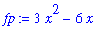
The
D
command acts like the differentiation operator in that it computes the derivative of a function and returns a function.
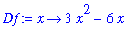
Note that the latter form is more convenient when it will be necessary to compute the derivative at a specific point.
| > |
Df(1) = eval( fp, x=1 );
|

Higher-order derivatives are obtained by specifying additional arguments to the
diff
command or by composing
D
with itself an appropriate number of times.
| > |
diff( exp(a*x), x, x );
|


Applications of Derivatives
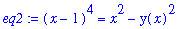
Implicit Differentiation
Implicit differentiation can be done in several different ways. Consider the implicitly defined function
| > |
impl_eq := (x-1)^4 = x^2 - y^2;
|
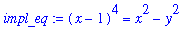
The
implicitdiff
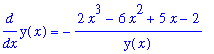
command can be used to find derivatives by implicit differentiation.
| > |
dy/dx = implicitdiff( impl_eq, y, x );
|
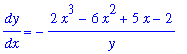
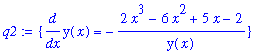
Observe that the second and third arguments define the dependence between the names -- the second argument is the dependent variable, the third argument is the independent variable.
The same result can be found by rewriting the implicit function to explicitly note the dependence of
 on
on

| > |
eq2 := eval( impl_eq, y=y(x) );
|
and differentiating the result with respect to
 .
.
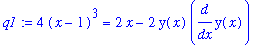
| > |
q2 := solve( q1, { diff(y(x),x) } );
|
These two commands can, of course, be combined into a single command.
| > |
impl_diff := diff( eval( impl_eq, y=y(x) ), x );
|
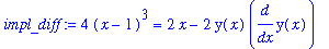
The formula for
 is obtained by solving the above equation for this quantity.
| > |
impl_dydx := isolate( impl_diff, diff(y(x),x) );
|
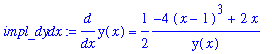
While this formula is not the same as either of the derivatives found earlier, it is easily seen to be an equivalent result.
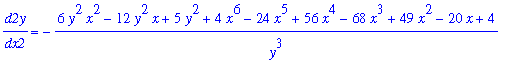
Higher-order implicit derivatives are obtained with
implicitdiff
by repeating the independent variable as many times as the desired order of the derivative (exactly as in
diff
).
| > |
d2y/dx2 = implicitdiff( impl_eq, y, x,x );
|
Compare this with the step-by-step computation of the same (we hope) result with
diff
:
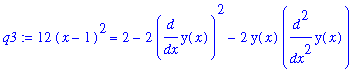
| > |
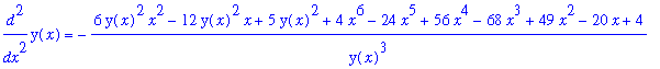
q4 := solve( q3, { diff(y(x),x,x) } );
|
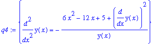
| > |
lhs(q4[]) = simplify( eval( rhs(q4[]), q2 ) );
|
Linearization of a Function
| > |
with( Student[Calculus1] ):
|
The linearization of a function
 at
at
 is
is
 + f'(
+ f'(
 ) (
) (
 ). For example, if
and

the linearization of f at
 can be obtained with the
TaylorApproximation
command from the
Student[Calculus1]
package as follows:
can be obtained with the
TaylorApproximation
command from the
Student[Calculus1]
package as follows:
| > |
TaylorApproximation( f(x), x=a );
|

The
unapply
command can be sued to convert this into a function
| > |
L1 := unapply( TaylorApproximation( f(x), x=a ), x );
|
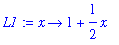
An alternate definition of this linearization is
| > |
L2 := x -> f(a) + D(f)(a)*(x-a);
|

The difference in the output is caused by the fact that Maple does not fully evaluate the right-hand side of the arrow operator (
->
) until the function is actually called. What this means is that if either the function f or the point
 are changed, then the function
L2
will reflect those changes as well. The function
L1
, however, uses the values of f and
are changed, then the function
L2
will reflect those changes as well. The function
L1
, however, uses the values of f and
 at the time the command is executed
and is unaffected by subsequent changes. This is illustrated in the following examples.
at the time the command is executed
and is unaffected by subsequent changes. This is illustrated in the following examples.

The function and its linearization can be graphed as follows.
| > |
TaylorApproximation( f(x), x=a, output=plot );
|
![[Maple Plot]](images/maple8-overview256.gif)
To determine the largest interval on which the linearization differs from the original function by no more than a specified amount,
i.e.
, to estimate the largest
 such that
 <
<
 implies
 <
<
 , we first look at the graph
| > |
plot( [ abs( f(x)-L2(x) ), epsilon ], x = 0 .. 3 );
|
![[Maple Plot]](images/maple8-overview262.gif)
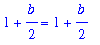
Click the left mouse button as close as possible to the leftmost of the two intersections of the curves in the plot. The box at the left end of the context bar shows the approximate coordinates of this point; this gives the point ( 0.57, 0.01 ). Repeating this process for the rightmost intersection gives ( 1.49, 0.01 ). This gives the estimate
 = min( 1-0.57, 1.49-1 ) = 0.43.
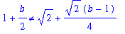
More accurate estimates of the intersection points will give more accurate estimates for
 . In this case Maple can solve the inequality
 .
.
| > |
solve( abs( f(x)-L2(x) ) < epsilon, x );
|

This yields
| > |
delta := min( 1-0.5526014252, 1.503967117-1 );
|
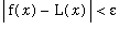
To conclude, check that the error never exceeds
 over this interval.
| > |
plot( [ abs( f(x)-L2(x) ), epsilon ], x = 1-delta .. 1+delta );
|
![[Maple Plot]](images/maple8-overview269.gif)
Newton's Method
| > |
with( Student[Calculus1] ):
|
Newton's Method is implemented with the
NewtonsMethod
command (from the
Student[Calculus1]
package). For example, consider the problem of finding the solution closest to
 , accurate to five decimal places, to
 when
when
| > |
f := x -> cos( 5*x ) - x:
|
Define the initial guess

Apply one iteration of Newton's Method to obtain
| > |
x1 := NewtonsMethod( f(x), x=x0, iterations=1 );
|
Additional iterations of Newton's Method yield
| > |
x2 := NewtonsMethod( f(x), x=x1, iterations=1 );
|
| > |
x3 := NewtonsMethod( f(x), x=x2, iterations=1 );
|

| > |
x4 := NewtonsMethod( f(x), x=x3, iterations=1 );
|
Thus,
 is an approximate value of the root closest to
 . If this process had continued too much longer, it would be more efficient to use the following loop to compute the iterates. (See the online help for
do .. end do
.)
. If this process had continued too much longer, it would be more efficient to use the following loop to compute the iterates. (See the online help for
do .. end do
.)
![x[0] := -1](images/maple8-overview279.gif)
| > |
x[1] := NewtonsMethod( f(x), x=x[0], iterations=1 );
|
![x[1] := -.7784735010](images/maple8-overview280.gif)
| > |
for n from 2 while abs( x[n-1] - x[n-2] ) >= 10^(-6) do
|
| > |
x[n] := NewtonsMethod( f(x), x=x[n-1], iterations=1 );
|
![x[2] := -.7677474241](images/maple8-overview281.gif)
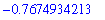
![x[3] := -.7674935683](images/maple8-overview282.gif)
![x[4] := -.7674934212](images/maple8-overview283.gif)
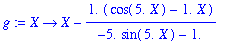
The explicit function used for one iteration of Newton's Method can be defined with
| > |
g := unapply( NewtonsMethod( f(x), x=X, iterations=1 ), X );
|
A sequence of Newton iterates can be obtained by adding
output=sequence
:
| > |
NewtonsMethod( f(x), x=-1, iterations=3, output=sequence );
|

If the
iterations
argument is omitted, then 5 iterations are performed.
| > |
NewtonsMethod( f(x), x=-1, output=sequence );
|

If the
output=sequence
argument is also omitted, then only the fifth iteration is returned
| > |
NewtonsMethod( f(x), x=-1 );
|
To conclude this discussion, using
output=plot
produces in a graphical display of the Newton iterations.
| > |
NewtonsMethod( f(x), x=-1, output=plot, iterations=3 );
|
![[Maple Plot]](images/maple8-overview288.gif)
Notice how each step of the Newton iteration uses the tangent line to the curve at the current iteration to obtain the next iteration. (To understand the hypotheses for the convergence theorem for Newton's method, think about what would happen if one of the tangent lines was horizontal, or nearly horizontal.)
Definite, Indefinite, and Improper Integrals
The
int
command is used to compute integrals in Maple. The indefinite integral
 is obtained with the command
Note that it is necessary to explicitly include the constant of integration,
 .
.
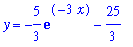
If additional information is given, it should be possible to determine a specific value for
 . For example, Maple can be used to find the function that satisfies the initial value problem
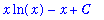
y'(x) =


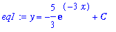
First, find the antiderivative (don't forget to include the constant of integration)
| > |
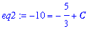
eq1 := y = int( 5*exp(-3*x), x ) + C;
|
To determine the appropriate value of
 , apply the initial condition
| > |
eq2 := eval( eq1, { y=-10, x=0 } );
|
and solve for

| > |
eq3 := C = solve( eq2, C );
|
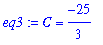
The solution to the initial value problem is
The
Student[Calculus1]
package contains a number of commands for the visualization and estimation of Riemann sums.
| > |
with( Student[Calculus1] ):
|
To illustrate, consider the problem of approximating the value of
 . Let
. Let

The midpoint approximation to this integral with 6 subdivisions is the area of the rectangles displayed with the
ApproximateInt
command
| > |
ApproximateInt(f, x=1..2, method=midpoint, partition=6, output=plot);
|
![[Maple Plot]](images/maple8-overview303.gif)
Observe that this plot displays the value of the corresponding Riemann sum (4.73958332) and the value of the definite integral (4.75). The explicit Riemann sum for this example can be obtained with
| > |
ApproximateInt(f, x=1..2, method=midpoint, partition=6, output=sum);
|
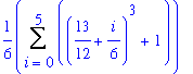
The value of this Riemann sum can be obtained as either

or
| > |
ApproximateInt( f, x=1..2, method=midpoint, partition=6 );
|

The floating-point approximation to this value is

An animation showing the convergence of a Riemann sum, or other quadrature method, can be obtained as follows:
| > |
ApproximateInt( f, x=1..2, output=animation,
method=random, subpartition=all, refinement=random,
partition=2, iterations=8 );
|
![[Maple Plot]](images/maple8-overview308.gif)
For other Riemann sums, change the
method
option to
right
,
left
,
random
,
upper
,
lower
, or
random
. For the Trapezoidal and Simpson's Rules, use
method=trapezoid
or
method=simpson
, respectively.
| > |
ApproximateInt(f, x=1..2, method=trapezoid, partition=4, output=plot);
|
![[Maple Plot]](images/maple8-overview309.gif)
The exact value of the definite integral is


While Maple is designed to be able to automatically evaluate many integrals, it can also be used to assist with techniques including substitution and integration by parts. The explicit commands implementing this capability are quite complex. But, they are easy to use in the form of the
Differentiation
maplet [
MapletViewer] [
MapleNet].
Applications of Integrals
Arclength of a Smooth Curve
| > |
with( Student[Calculus1] ):
|
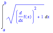
The definite integral for the arclength of a smooth curve is usually easy to formulate but difficult to evaluate. The general formula for the arclength of the graph of
 for
for
 in
in
![[a, b]](images/maple8-overview314.gif) is
is
| > |
ArcLength( f(x), x=a .. b, output=integral );
|
For example, with
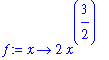
on the interval [ 0, 1 ], the definite integral for the arclength is
| > |
ArcLength( f(x), x=0..1, output=integral );
|
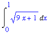
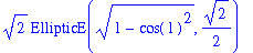
The exact value of this integral is
| > |
ArcLength( f(x), x=0..1 );
|

Maple is able to evaluate many more integrals than most humans, but there are many arclength integrals that cannot be evaluated explicitly. If this occurs, or if Maple's answer involves functions that are not familiar to you, use
evalf
to force a numerical approximation of the integral.

| > |
ArcLength( f(x), x=0..1 );
|

Improper Integrals
Improper integrals are not a problem for Maple. Here are three examples.
| > |
int( x * exp(-x), x = 1 .. infinity );
|

| > |
int( 1/sqrt(4-x^2), x = 0 .. 2 );
|

| > |
int( 1/x, x = 1 .. infinity );
|

Multiple Integrals
The
int
and
Int
commands can be used to construct iterated integrals corresponding to double and triple integrals.
| > |
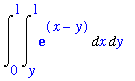
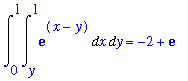
Int( Int( exp(x-y), x = y .. 1 ), y = 0 .. 1 );
|
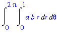
The area of the ellipse
 can be found by parameterizing the ellipse in polar coordinates:
 ,
,
 with 0 <=
 <= 1 and 0 <=
 <
<
 . The Jacobian of this change of variables is
 , so the area of the ellipse is
| > |
Int( Int( a*b*r, r = 0 .. 1 ), theta = 0 .. 2*Pi );
|
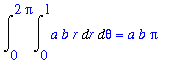
Note that this result reduces to the familiar area of a circle when
 .
.
Maple and Differential Equations
The
dsolve
command attempts to solve a differential equation. If initial conditions are provided, a particular solution is sought; otherwise, the successful result will be the general solution.
| > |
ode := diff( y(x), x ) = y(x) * (3-y(x)) * (x-1);
|
| > |
soln := dsolve( ode, y(x) );
|
Note that Maple has returned the general solution to this differential equation. The name
_C1
is the parameter for this one-dimensional family of solutions.
To find the solution that passes through a specific point, substitute the initial condition into the solution, solve for
_C1
, and substitute the result back into the general solution:
| > |
q1 := eval( soln, { y(x) = 2, x=0 } );
|
| > |
q2 := solve( q1, { _C1 } );
|
| > |
q3 := eval( soln, q2 );
|

If the particular solution to an initial value problem is all that is needed, then the above process can be streamlined to a single
dsolve
command in which the first argument is a
set
containing the differential equation and the initial condition.
| > |
q4 := dsolve( { ode, y(0)=2 }, y(x) );
|
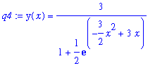
Notice that the solution returned by
dsolve
is an equation. To plot this solution, use the
rhs
command to pass only the right-hand side of the solution to the
plot
command.
| > |
plot( rhs(q4), x=-1..4 );
|
![[Maple Plot]](images/maple8-overview343.gif)
The
DEtools
package contains a number of useful commands for working with differential equations.


In particular, the
DEplot
command can be used to display a direction field and/or solution curves for a differential equation.
| > |
DEplot( ode, [y(x)], x=-1..4, [ [0,2] ], arrows=none );
|
![[Maple Plot]](images/maple8-overview355.gif)
Changing the last argument to
arrows=thin
will include the direction field. Adding additional ordered pairs to the list of initial conditions will add additional solution curves to the plot. The online help for
DEplot
describes other options that control features such as the color of the arrows and solution curves, the window for the plot, and the stepsize.
| > |
init_cond := [ [0,0], [0,1], [0,2], [0,3] ];
|
![init_cond := [[0, 0], [0, 1], [0, 2], [0, 3]]](images/maple8-overview356.gif)
| > |
DEplot( ode, [y(x)], x=-1..4, init_cond, arrows=thin );
|
![[Maple Plot]](images/maple8-overview357.gif)