Piecewise linear basis functions

Piecewise linear basis functions provide a good compromise between accuracy and computational cost due to their bounded support. The Sparse Grid Interpolation package includes three different grid types that work with piecewise multilinear basis functions:

The Clenshaw-Curtis grid type "ClenshawCurtis" (CC)
the "classical" maximum-norm-based grid type "Maximum" (M), as described e.g. by Bungartz/Griebel in [1],
The maximum-norm-based grid without points on the boundary "NoBoundary" (NB), with basis functions that extrapolate towards the boundary (it is not assumed that the objective function must be zero at the boundary).

For a detailed description of the piecewise multilinear basis functions implemented here, please see [2] or [3, ch. 3], and the references stated therein.

Accuracy of piecewise multilinear interpolation

We now take a brief look at the approximation quality. An a priori error estimate can be obtained for a d-variate function f if continuous mixed derivatives

with

exist. According to [4] or [5], the order of the interpolation error in the maximum norm is then given by

where A_q,d(f) denotes the sparse grid interpolant of f, and N denotes the number of grid points of the sparse grids of type CC or M (the NB grid type has not yet been analyzed, but shows the same order of convergence in numerical tests). Note that the number of grid points N of A_q,d(f) can be computed by spdim(q-d,d). Piecewise multilinear approximation on a full grid with N^* grid points is much less efficient, i.e. O(N^*^-2/d).

Number of grid points

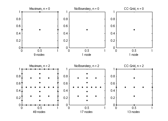
The following table shows the number of grid points of the non-adaptive sparse grid interpolant depending on the interpolation depth n.

n d=2 d=4 d=8

M NB CC M NB CC M NB CC

0 9 1 1 81 1 1 6561 1 1

1 21 5 5 297 9 9 41553 17 17

2 49 17 13 945 49 41 1.9e5 161 145

3 113 49 29 2769 209 137 7.7e5 1121 849

4 257 129 65 7681 769 401 2.8e6 6401 3937

5 577 321 145 20481 2561 1105 9.3e6 31745 15713

6 1281 769 321 52993 7937 2929 3.0e7 141569 56737

7 2817 1793 705 1.3e5 23297 7537 9.1e7 5.8e5 1.9e5

n	d=2	d=4	d=8
	M	NB	CC	M	NB	CC	M	NB	CC
0	9	1	1	81	1	1	6561	1	1
1	21	5	5	297	9	9	41553	17	17
2	49	17	13	945	49	41	1.9e5	161	145
3	113	49	29	2769	209	137	7.7e5	1121	849
4	257	129	65	7681	769	401	2.8e6	6401	3937
5	577	321	145	20481	2561	1105	9.3e6	31745	15713
6	1281	769	321	52993	7937	2929	3.0e7	141569	56737
7	2817	1793	705	1.3e5	23297	7537	9.1e7	5.8e5	1.9e5

The following graph illustrates the sparse grids of level 0 and level 2 of the three respective grids in two dimensions.

Which piecewise linear interpolation scheme works best?

Although the performance of the three grid types is rather similar for lower-dimensional problems, there are two important points to be mentioned:

The ClenshawCurtis grid and the NoBoundary grid have just a single node at the lowest interpolation level n = 0 (this means that an interpolant of level 0 of these grid types is just a constant function). The Maximum grid has 3^d nodes at the lowest level. Therefore, the Maximum is not well-suited for higher-dimensional problems. For instance, for d = 10, already 59049 support nodes would be required to obtain an initial interpolant.
Since the CC-grid is the most versatile grid working well in both lower and higher dimensions, at this point, the dimension-adaptive algorithms are implemented for this grid type only.

Therefore, for most practical applications, we recommend using the Clenshaw-Curtis grid. Occasionally, the other grid types may perform better by a small factor, as numerical experiments show (try running the demo spcompare from the command line or from the Sparse Grid Interpolation demo page).