pdepe_test

pdepe_test, MATLAB programs which illustrate how to use the MATLAB command pdepe(), which can solve initial boundary value problems (IBVP's) in one spatial dimension.

Example of a 1D Initial Boundary Value Problem:

The classic example of such a problem is the time-dependent heat equation posed on a line segment [a,b]:

        ODE: d/dt u(x,t) - d/dx a(x,t) d/dx u(x,t) = f(x,t)
        IC:  u(x,0) = u0(x)
        BC:  u(a,t) = g(t)
             u(b,t) = h(t)

Here,

u(x,t) is the temperature measured at a point x at time t;
a(x,t) is the thermal conductivity, which might be a constant, or a function only of space, or of both space and time;
f(x,t) is a source term that might be 0, constant, or a varying function.
u0(x) is the initial condition, that is, the value of the temperature at all points in the interval, at an initial time, usually taken to be t=0.
g(t) and h(t) are functions which declare the values of the solution at the left and right endpoints, which are often fixed values. The boundary conditions listed here are of Dirichlet type, because they specify the value of the solution itself. It is also possible to set one or both boundary conditions to be of Neumann type, in which case we provide a formula for the spatial derivative du/dx for all time at the boundary point.

A solution to this 1D boundary value problem is a formula for u(x,t), or, more realistically, a table of values for u(x,t) at selected times and points. For the heat equation, there are many procedures for coming up with a table of good approximations to the solution. The advantage of using MATLAB's pdepe() is that it can provide this solution automatically, that is, your only work is to provide the information that defines the problem. You hand this information to pdepe(), and it hands you back the solution.

1D Initial Boundary Value Problems that PDEPE Can Solve:

The simplest version of the pdepe() command has the form:

        sol = pdepe ( m, pdefun, icfun, bcfun, xmesh, tspan )

The input parameters have the following meanings:

m chooses Cartesian (0), cylindrical(1), or spherical geometry(2);
pdefun() is an M-file that defines the partial differential equation;
icfun() is an M-file that defines the initial conditions;
bcfun() is an M-file that defines the boundary conditions;
xmesh is a vector of spatial coordinates where the solution is desired.
tspan is a vector of times at which the solution is desired.

and the output is:

u(:,:,:), the solution. u(i,j,k) is the value at the i-th time, the j-th spatial coordinate, of the k-th coordinate of the solution.

The pdepe() function thinks of the equation to be solved as

        c() * du/dt = 1/x^m d/dx ( x^m f() ) + s()

The variable u may be a scalar or a vector. If u is a vector, then so are the quantities c(), f(), and s().

In the typical case, c() is 1, and m is 0. Moreover, c(), f() and s() are functions of x, t, u, and du/dx. That means that a simple version of the heat equation such as:

        ut - d/dx ( sin(x) * du/dx ) = x^2

can be put into the pdepe() format by prescribing:

        c = 1.0;
        f = sin(x) * dudx;
        s = x^2;

The pdefun() function must have the form:

        [ c, f, s ] = pdefun ( x, t, u, dudx )

Here, the input is

x, a point in the domain;
t, the current time;
u(), the current solution (scalar or vector);
dudx(), the current solution spatial derivative (scalar or vector);

The output to be computed by pdefun() is a set of three items, which are scalar if u() is a scalar, or column vectors if u() is a vector:

c(:), the coefficients of du/dt;
f(:), the term to which d/dx is to be applied.
s(:), the source term.

The icfun() function must have the form:

        u = icfun ( x )

Here, the input is

x, a point in the domain;

and the output is

u, the value of the solution at position x and time t0.

The pdepe() function models the boundary conditions as:

        pl ( x, t, u ) + ql ( x, t, u ) * f ( x, t, u, dudx ) = 0  at x = xl;
        pr ( x, t, u ) + qr ( x, t, u ) * f ( x, t, u, dudx ) = 0  at x = xr.

The pl/pr functions take care of Dirichlet boundary conditions, while the ql/qr functions take care of flux or Neumann conditions. For example, to impose the condition:

        u(xl) = 7
        2 * u(xr) + sin ( xr ) * dudx ( xr ) = sqrt ( t )

assuming that f(x,t,u,dudx) is defined to be dudx, we simply set:

        pl = ur - 7.0;
        ql = 0.0;
        pr = 2.0 * ur - sqrt ( t );
        qr = sin ( xr );

The bcfun() function must have the form:

        [ pl, ql, pr, qr ] = bcfun ( xl, ul, xr, ur, t )

Here, the input is

xl, the location of the left endpoint;
ul, the solution at the left endpoint;
xr, the location of the right endpoint;
ur, the solution at the right endpoint;
t, the current time;

and the output is

pl, the value of p at the left endpoint.
ql, the value of q at the left endpoint.
pr, the value of p at the right endpoint.
qr, the value of q at the right endpoint.

Licensing:

The computer code and data files described and made available on this web page are distributed under the GNU LGPL license.

Languages:

PDEPE is available in a MATLAB version.

Related Data and Programs:

BVP4C, MATLAB programs which illustrate how to use the MATLAB command bvp4c(), which can solve boundary value problems (BVP's) in one spatial dimension.

Reference:

http://www.mathworks.com/help/matlab/pdepe.html , the MathWorks help page for PDEPE.
P Howard,
Differential Equations in Matlab 7.0,
Spring 2005.

Examples and Tests:

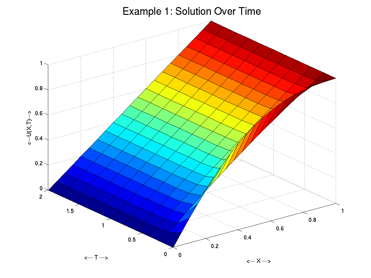
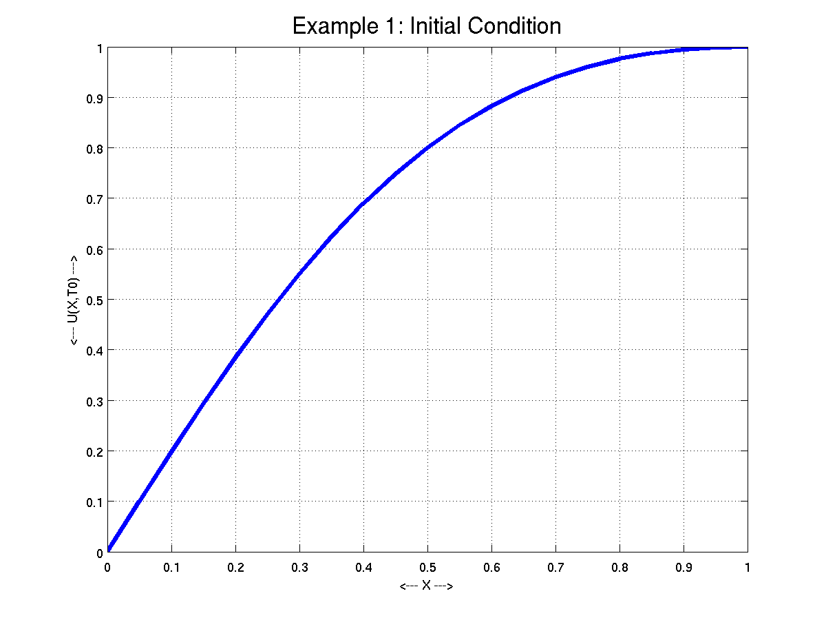
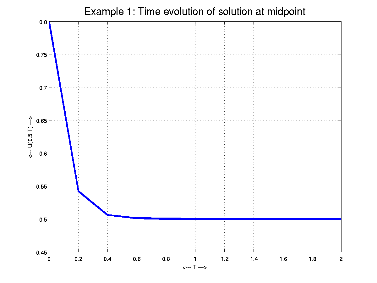
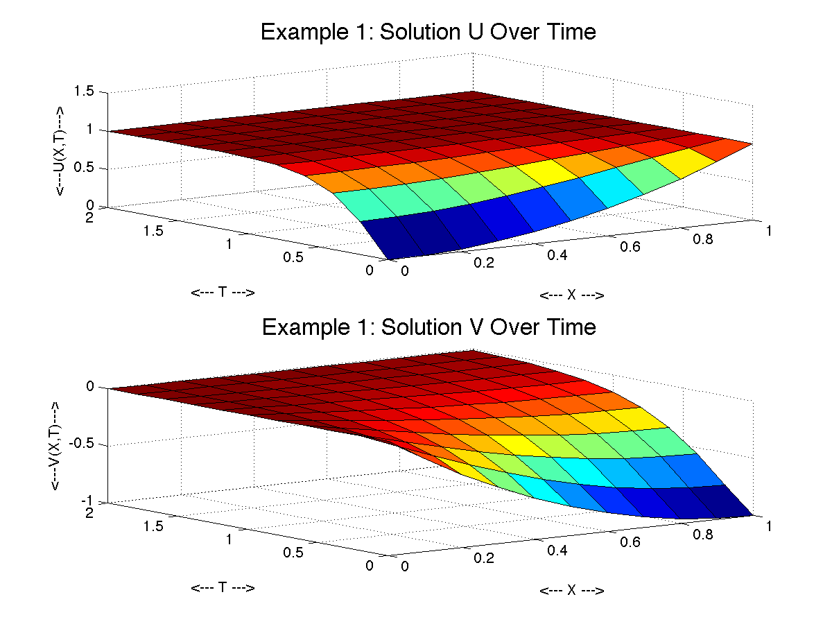
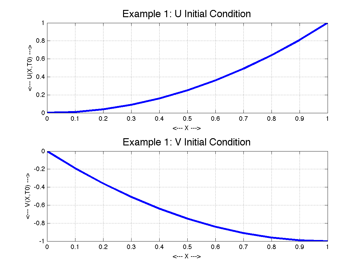
Example 1 is a version of the heat equation.

example1.m, defines the problem, calls pdepe() to solve it, and plots the results.
example1.png, a surface plot of the solution U(X,T).
example1_ic.png, a line plot of the initial condition U(X,T0).
example1_profile.png, a line plot of the solution at a fixed point, U(midpoint,T).

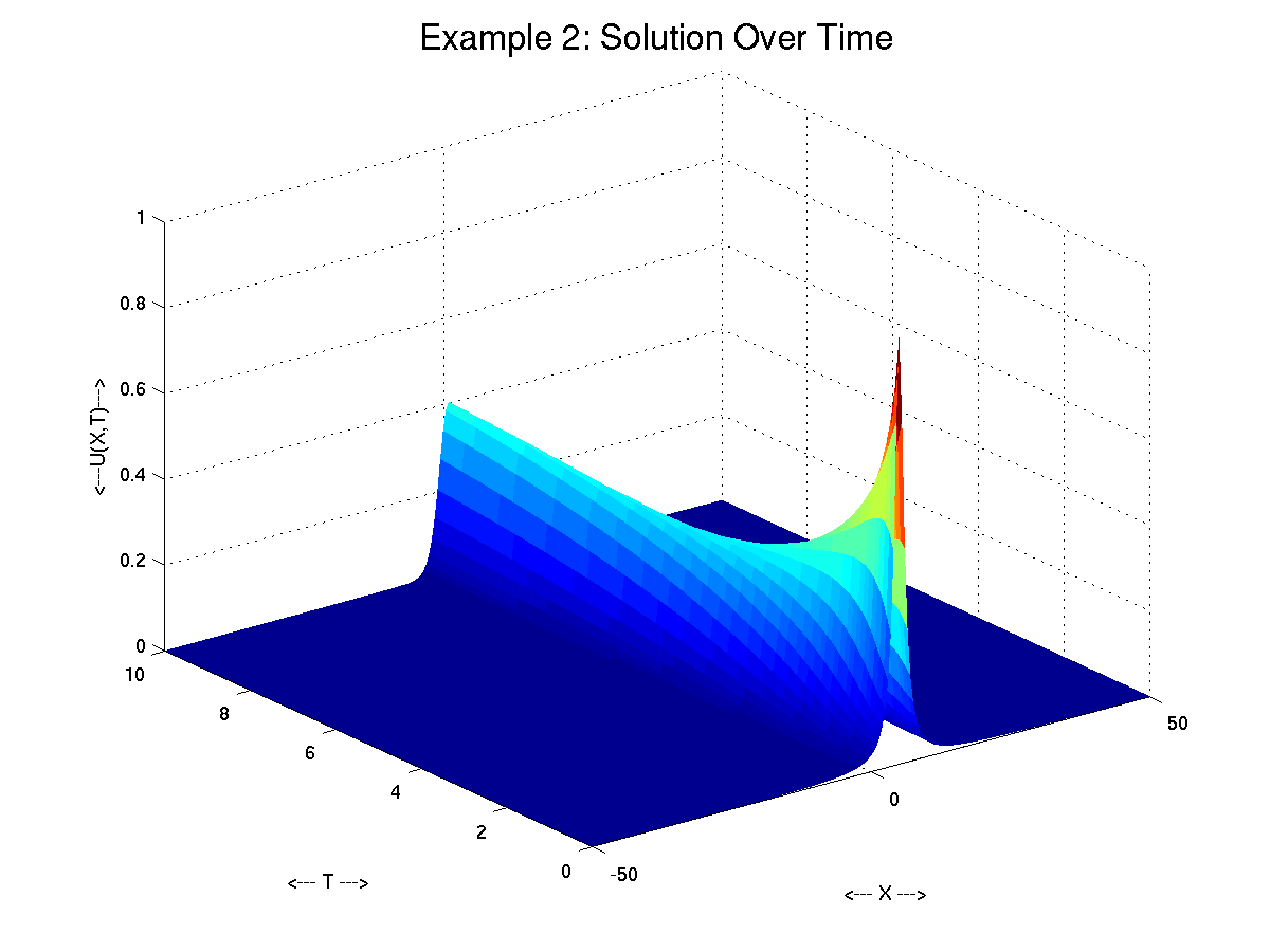
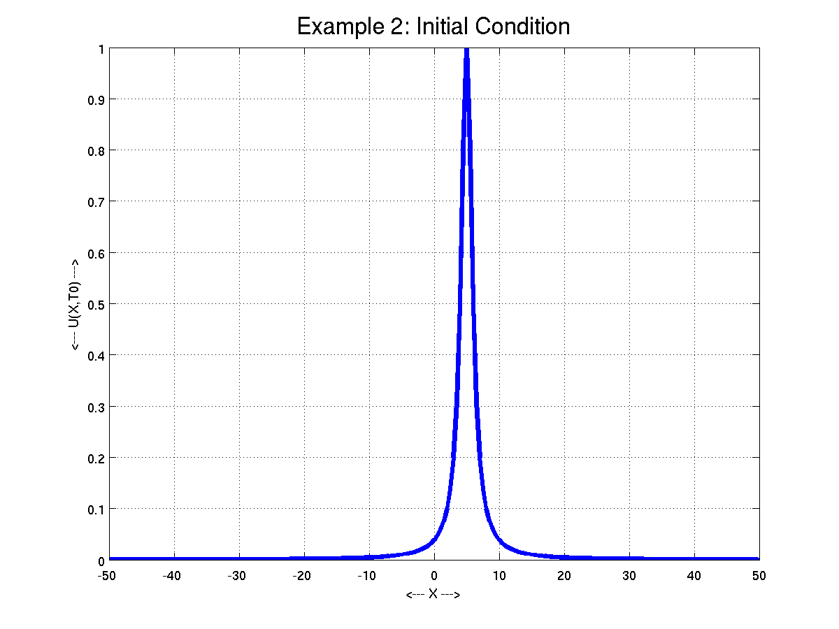
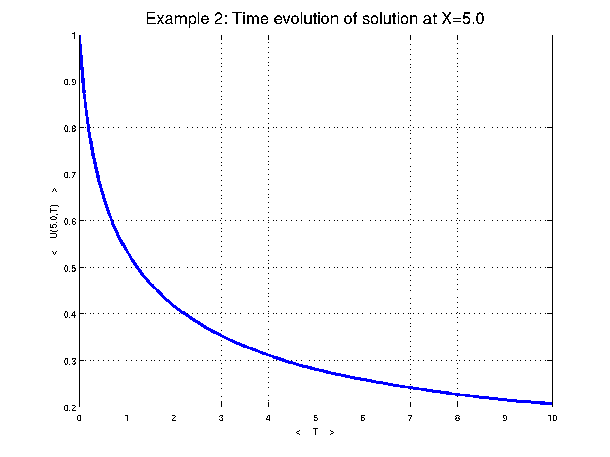
Example 2 is a version of the convection-diffusion equation, with a variable coefficient.

example2.m, defines the problem, calls pdepe() to solve it, and plots the results.
example2.png, a surface plot of the solution U(X,T).
example2_ic.png, a line plot of the initial condition U(X,T0).
example2_profile.png, a line plot of the solution at a fixed point, U(5.0,T).

Example 3 is a nonlinear predator prey system for the two variables [u,v].

example3.m, defines the problem, calls pdepe() to solve it, and plots the results.
example3.png, a surface plot of the solutions U(X,T), V(X,T).
example3_ic.png, a line plot of the initial condition U(X,T0), V(X,T0).
example3_profile.png, a line plot of the solution at a fixed point, U(0.5,T), V(0.5,T).

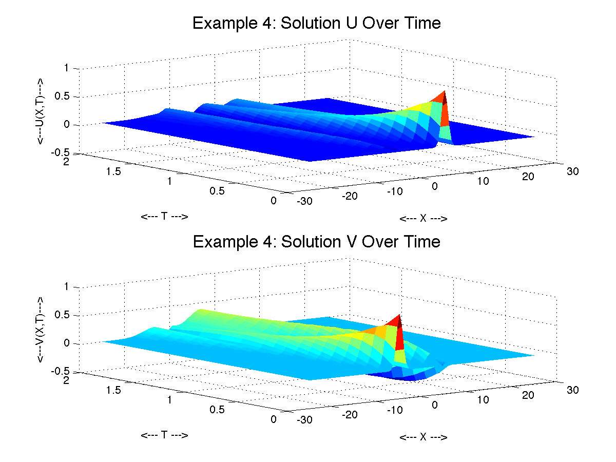
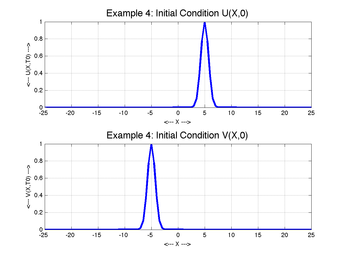
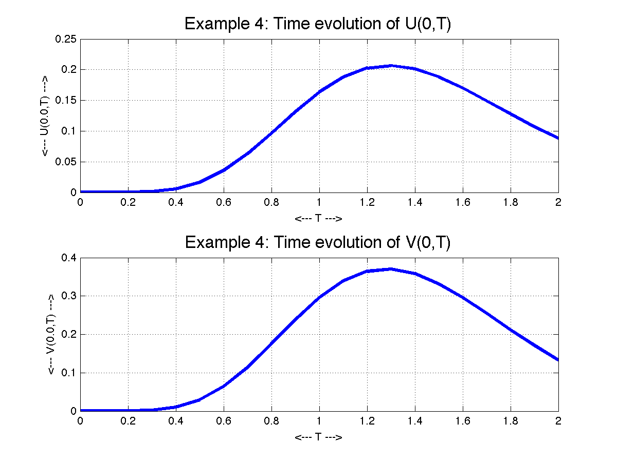
Example 4 is a system of convection-diffusion equations with variable coefficient.

example4.m, defines the problem, calls pdepe() to solve it, and plots the results.
example4.png, a surface plot of the solutions U(X,T), V(X,T).
example4_ic.png, a line plot of the initial conditions U(X,T0), V(X,T0).
example4_profile.png, a line plot of the solutions at a fixed point, U(0.0,T), V(0.0,T).

You can go up one level to the MATLAB source codes.

Last revised on 06 September 2013.