GPL is a data directory which contains examples of GPL files, that is, text files which can be read and displayed by GNUPLOT.
A 1D GPL data file can be created for processing by the gnuplot "plot" command:
        gnuplot
          set style data lines
          plot 'myfile.gpl'
In the simplest case, the user simply has a consecutive sequence of values, which are displayed as the Y coordinates of equally spaced X locations.
A 2D GPL data file can be created for processing by the gnuplot "plot" command:
        gnuplot
          set style data lines
          plot 'myfile.gpl'
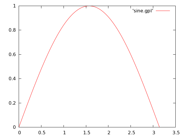
In the simplest case, the user wishes to draw a single curve by connecting N pairs of (X,Y) points, and the GPL file contains N consecutive lines of coordinate information. (Hash marks are allowed as comments.)
Thus, the file "sine.gpl" contains 101 lines of data, containing the values of sine(x) for x = 0 to Pi, and begins like this:
# sine.gpl
#  101 pairs of values (x,sin(x)) for x = 0 to pi.
#
         0         0
    0.0314    0.0314
    0.0628    0.0628
    0.0942    0.0941
    0.1257    0.1253
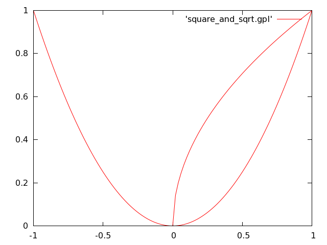
Suppose you wanted to draw two curves on a single plot, from data in a single file? And suppose the two curves did not use the same set of x values? This is no problem. Your GPL file simply lists the data for the first curve, followed by one blank line, and then the data for the second curve. We'll plot y = x^2 from -1 to 1, and y = sqrt(x) from 0 to 1 this way. The file square_and_sqrt.gpl looks like this:
# square_and_sqrt.gpl
#   y=x^2 and y=sqrt(x)
#
   -1.0000    1.0000
   -0.9800    0.9604
   -0.9600    0.9216
    ... more data for y=x^2...
    0.9800    0.9604
    1.0000    1.0000

         0         0
    0.0200    0.1414
    ... more data for y = sqrt(x)...
To make a PNG version of the Gnuplot image, use commands like this:
        gnuplot
          set term png
          set output 'sine.png'
          set style data lines
          plot 'sine.gpl'
          quit
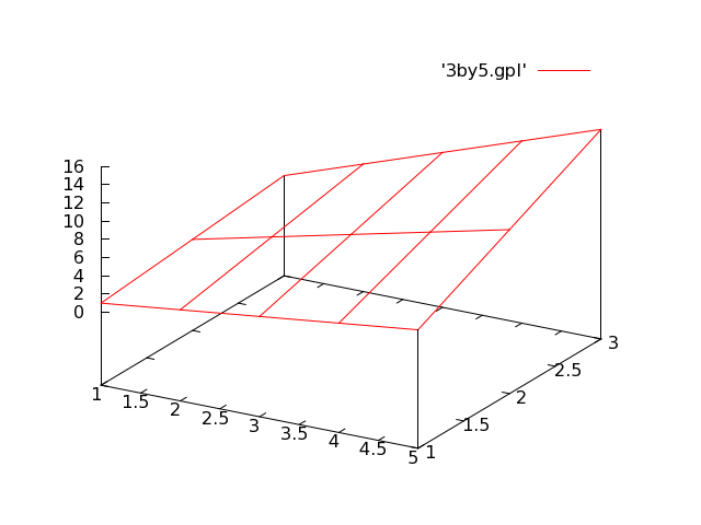
A very common plotting problem arises when we have a regular grid of M*N points (X,Y), on which we have function values Z(X,Y). One way of presenting such data is as a surface plot, so that the graph appears as a sort of hill. It is easy to set up a GPL file containing the data in such a way that GNUPLOT will automatically draw the desired surface.
Suppose that we have a very simple grid of 15 data points, defined by 5 X values and 3 Y values, as suggested by this sketch:
         1,3  2,3  3,3  4,3  5,3
         1,2  2,2  3,2  4,2  5,2
         1,1  2,1  3,1  4,1  5,1
and that the function we have is Z = X * Y.
A GPL data file can be created by listing the X, Y, and Z values for each point along the lowest value of Y. Then insert a space, and list the data for the next value of Y, and so on. Our entire GPL file for this example might be:
      # 5by3.gpl
      #
        1  1   1
        2  1   2
        3  1   3
        4  1   4
        5  1   5

        1  2   2
        2  2   4
        3  2   6
        4  2   8
        5  2  10

        1  3   3
        2  3   6
        3  3   9
        4  3  12
        5  3  15
The GNUPLOT splot command will automatically realize that we want
to draw a line in 3D space corresponding to each list of 5 values.
This would give us an image that looked like slices along the X
direction only. But GNUPLOT will also realize that there is a
pattern of 3 sets of such lists, and so it will also draw lines
connecting data in the Y direction, giving us the appearance of a surface.
To plot such data, we simply say
        gnuplot
          set style data lines
          splot '5by3.gpl'
To make a PNG version of the Gnuplot image, use commands like this:
        gnuplot
          set term png
          set output '5by3.png'
          set style data lines
          plot '5by3.gpl'
          quit
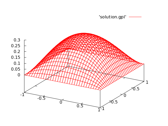
A finite element program like DEAL.II may start with a simple grid, like that used by the 3by5 example. However, as the calculation seeks greater accuracy, it may subdivide some squares into 4 smaller squares, and this may happen repeatedly, and to various levels over the grid. In the end, the region has been broken up into squares of many different sizes, and the answer is reported by listing, for each such square, the X,Y,Z values of the four vertices, where here the Z value is the value of some quantity computed by the program, so that we have a functional form Z=Z(X,Y).
We can still use a GPL file to store this data, but now we have to essentially treat each square as a separate subplot, that is, as a 2 by 2 grid! A square is therefore described by 5 lines of text, that is, two sets of (X,Y,Z) data for one side, a blank line, and then two more sets of (X,Y,Z) data.
How do we plot multiple squares? We simply follow this data by two blank lines, and then the data for the next square. We can repeat this as many times as we need to. Then the same commands that worked for the 3by5 example can be used to plot our finite element solution.
The file "solution.gpl" was created by DEAL.II. It turns out that no subdivision was carried out, so the information is actually on a completely regular grid. However, the data file is written in the general format, and begins this way:
# This file was generated by the deal.II library. # Date = 2013/7/5 # Time = 10:50:42 # # For a description of the GNUPLOT format see the GNUPLOT manual. # #-1 -1 0 SQUARE 1 VERTEX 1 (left bottom) -0.9375 -1 0 SQUARE 1 VERTEX 2 (right bottom) 1 line separates sides of square 2 -1 -0.9375 0 SQUARE 1 VERTEX 3 (left top) -0.9375 -0.9375 0.00812348 SQUARE 1 VERTEX 4 (right top) 2 lines separate square 1 from square 2 2 lines separate square 1 from square 2 -0.9375 -1 0 SQUARE 2 VERTEX 1 (left bottom) -0.875 -1 0 SQUARE 2 VERTEX 2 (right bottom) 1 line separates sides of square 2 -0.9375 -0.9375 0.00812348 SQUARE 2 VERTEX 3 (left top) -0.875 -0.9375 0.0140283 SQUARE 2 VERTEX 4 (right top) 2 lines separate square 2 from square 3 2 lines separate square 2 from square 3 -1 -0.9375 0 SQUARE 3 VERTEX 1 (left bottom) ...and so on...
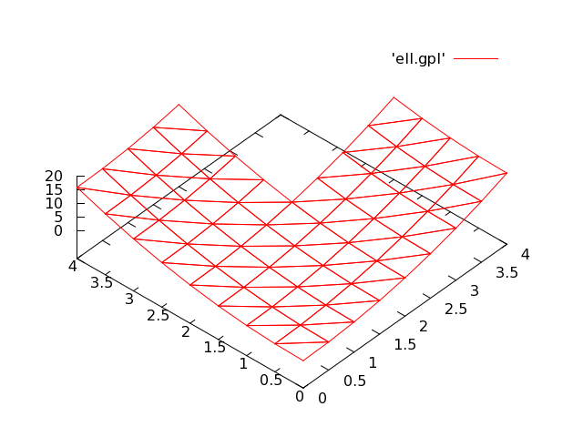
Most finite element programs use triangles, rather than squares, when defining a grid for the solution. Thus, the GPL format must be modified if we have solution data organized as a list of triangles, for each of which we have the X,Y,Z values associated with each vertex, where Z of course is some function Z(X,Y) whose value was calculated by the finite element program.
To draw the outline of a single triangle, we simply have to list the (X,Y,Z) values of the vertices, repeating the first vertex at the end:
        x1 y1 z1
        x2 y2 z2
        x3 y3 z3
        x1 y1 z1
Now we actually have many triangles to draw. All we need to do is
insert two blank lines into the file before listing the next triangle,
and GNUPLOT will be able to display a 3D surface with any number of
triangles. Here is how the file "ell.gpl" begins:
#  ell.gpl
#  Data on triangles.
#
0.000000  0.000000  0.000000
0.500000  0.000000  0.250000
0.000000  0.500000  0.250000
0.000000  0.000000  0.000000


1.000000  0.000000  1.000000
0.500000  0.500000  0.500000
0.500000  0.000000  0.250000
1.000000  0.000000  1.000000


0.000000  1.000000  1.000000
The computer code and data files described and made available on this web page are distributed under the GNU LGPL license.
You can go up one level to the DATA page.