71.html

7th Funky Function:

A continuous, non-constant, differentiable function

whose derivative is zero everywhere

except on a set of Lebesgue measure zero.

The Maple Code on this page is from I.N. Galidakis

(http://ioannis.virtualcomposer2000.com/math/cantor.html).

Special thanks to him!

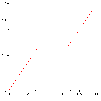
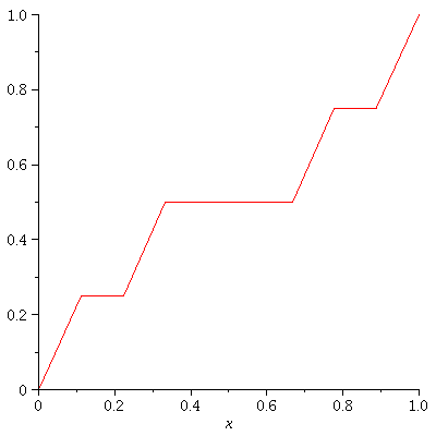
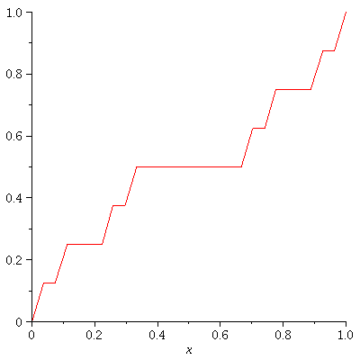
It's the Cantor Function f: [0,1] -> [0,1].

As explained at the Wiki link,

the Cantor function is the uniform limit

of a sequence {} of piecewise linear functions.

Let's graph

f_0, f_1, f_2, .... f_enough ,

each on it's own grid.

So we will have (enough+1) graphs.

> restart; with(plots):
enough := 3;
CF:=proc(a,b,c,d,n,x) option remember;
if n=0 then solve((d-c)/(b-a)=(y-c)/(x-a),y);
else #n>0
piecewise(a<=x and x<=a+1/3*abs(a-b),CF(a,a+1/3*abs(a-b),c,c+1/2*abs(c-d),n-1,x),
b-1/3*abs(a-b)<=x and x<=b, CF(b-1/3*abs(a-b),b,d-1/2*abs(c-d),d,n-1,x),
c+1/2*abs(c-d));
fi;
end:
for n from 0 to enough do
plot(CF(0,1,0,1,n,x),x=0..1,numpoints=300);
od;

Plot_2d

Plot_2d

Plot_2d

Plot_2d

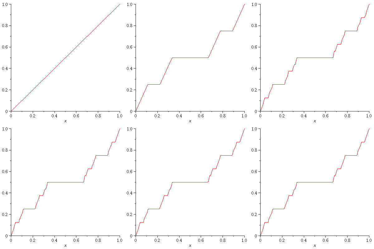
Next let's graph

f_0, f_1, f_2, .... f_enough

all on the same grid in a fancy

"animated" effect with the f_n's

forming a "moving picture". I set

the speed at 1 frame per second

so it will take (enough+1) seconds to show

you f_0 through f_enough

> restart; with(plots):
enough := 9;
CF:=proc(a,b,c,d,n,x) option remember;
if n=0 then solve((d-c)/(b-a)=(y-c)/(x-a),y);
else #n>0
piecewise(a<=x and x<=a+1/3*abs(a-b),CF(a,a+1/3*abs(a-b),c,c+1/2*abs(c-d),n-1,x),
b-1/3*abs(a-b)<=x and x<=b, CF(b-1/3*abs(a-b),b,d-1/2*abs(c-d),d,n-1,x),
c+1/2*abs(c-d));
fi;
end:
q1:=[seq(CF(0,1,0,1,n,x), n=0..enough)]:
q2:=[seq(plot(g,x=0..1),g=q1)]:
display(q2,insequence=true);

Plot_2d

That's all!